Comments Off on The Case for an Unconditional Safety Net
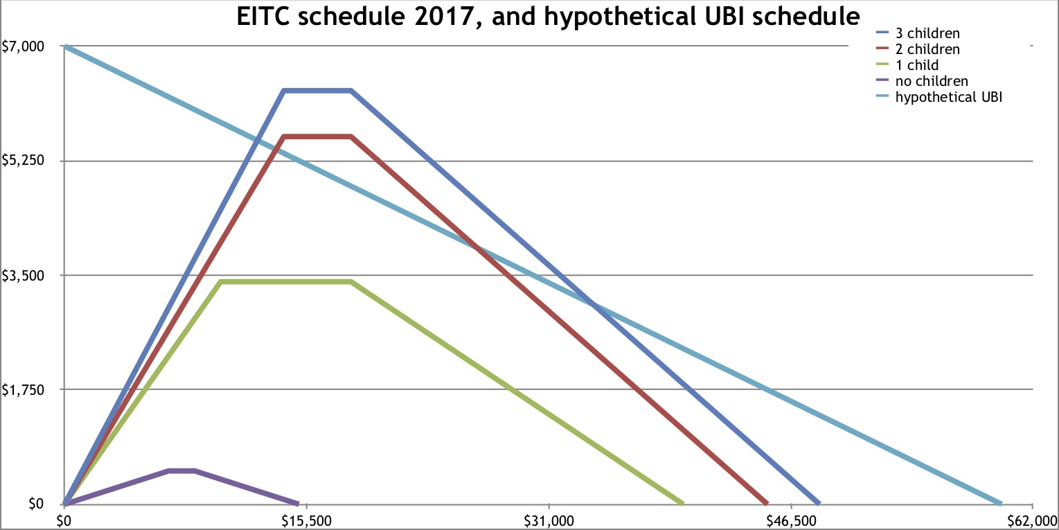
In the broader guaranteed income discourse, various tax and transfer schema are discussed as examples of both alternatives to a true UBI, and as case studies for examining the impact of cash transfers on social and labor market dynamics. As the single most progressive element of the U.S. tax code, the Earned Income Tax Credit (EITC) features prominently as a comparison object. Particularly politically popular because it both incentivizes work and targets families with children, the EITC is a refundable tax credit for low- to middle-income workers that begins at the first dollar of earned income and increases until phasing out at some maximum level. (For links to several studies of the EITC’s effects, see the third section of our ongoing cash transfers literature review.) A number of elected officials have recommended a significant expansion and modernization of the EITC—referred to by these lawmakers as a Cost-of-Living Refund—as a response the changing nature of work and the current limitations of the credit. Discussed modernizations include expanding the definition of work to include students and caregivers, increasing the total amount and expanding it its reach to the middle class, and establishing a monthly disbursement option.
In the below post, economist Max Kasy provides an accessible overview of a recent working paper, published with Data For Progress, in which he explores the limitations of the EITC and argues that an unconditional transfer system is preferable—economically, morally, and politically—to work-based benefits.
(Originally published at USBIG. Click here and here for further coverage of Kasy’s paper.)
Imagine a system where everyone had a right to basic material safety, and could say “no” to abuse and exploitation. Sounds utopian? In this article I argue that it would be quite feasible to get there, and that it would make eminent economic, moral, and political sense.
The Earned Income Tax Credit (EITC) is the most progressive component of the current U.S. income tax code, redistributing income toward families with low (but not without) earnings. The EITC was first introduced in 1975 and was substantially expanded in the 1990s. In order for someone to be eligible to receive EITC payments, they must have paid employment but earn less than a certain amount. Additionally, EITC payments go mostly to households with children. The combination of two key features makes the EITC a popular program among policymakers. First, the EITC significantly reduces poverty among working families. Second, it also provides a strong incentive for unemployed people to seek work.
But is a subsidy of low wage work, as provided by the EITC, really the best way to get money to people who need it? In a new working paper, I argue that it would be better to extend the benefits of the EITC to those who don’t have any income, rather than restricting them to low wage workers. Such a system could be based on an extension of the current EITC, providing transfers to those who don’t have any earnings, and then fading them out for households with moderate incomes. Such an extension would amount to a radical improvement of the lives of those at the bottom of the economic ladder, providing a basic safety net that would be available independently of the vagaries of life. It would provide an “outside option” that sets a floor to the conditions anyone has to accept, for material reasons, in relationships, jobs, or interactions with the government.
In my paper, I discuss four sets of arguments why it would make economic, moral, and political sense to transition from the current system of subsidizing low wage work to a system providing an unconditional safety net.
The economic arguments for a UBI are twofold: First, subsidies of low-wage work, such as an EITC, distort incentives; they cause people to work more than they otherwise would. Unconditional transfers would reduce the resulting inefficiency, so that there would be a bigger economic pie to distribute, and more money would go to those who need it.
In the paper, I call this the “magic bucket”: the idea that by moving from a world in which we provide subsidies of low-wage work to one in which we provide universal transfers, we incur societal savings. As we reduce conditional (EITC) payments to support an unconditional transfer system, individuals work less, which leads to government savings from fewer and smaller EITC transfers. As a result, you can reduce EITC payments by less than \$1 to pay for \$1 of unconditional transfers.
Second, subsidies of low-wage work depress wages. By providing incentives for people to work, such subsidies allow employers to pay less, so they are, at least in part, a transfer to employers rather than workers. Replacing subsidies of low-wage work with unconditional transfers would improve workers’ bargaining position and wages.
I also argue that there are important moral and political considerations for unconditional transfers over conditional ones, such as an EITC.
Unconditional transfers would increase individual liberty and would improve fairness. This sort of benefit would allow people in abusive relationships with domestic partners, employers, or government administrators to leave the situation without fear of material destitution. Unconditional benefits would also improve fairness by remunerating unpaid care work (particularly by women), civic engagement, and cultural production.
Lastly, unconditional transfers that are conceived of as a universal basic income would be politically more sustainable and popular than narrowly targeted transfers. Universal benefits tend to have stronger democratic support than conditional benefits for the poor (think Social Security or Medicare).
In summary, these arguments suggest that EITC benefits expanded to become a universal basic income would give more to those who need it, would promote liberty, and would be politically viable and stable.
If one accepts these arguments, a political case needs to be made for a UBI. Any such case must grapple with and overcome distinctions drawn between the “deserving” and the “undeserving” poor. Such distinctions underpin the popularity of conditional transfers among politicians, but that underpinning has historically often been based on racial discrimination. A case for a universal basic income also needs to provide alternative narratives of a shared fate and shared interests, of a common defense of liberty, and of the valuable contributions of those working outside paid labor.
U.S. politics is beset by increasing polarization. Ideological clustering is common; partisan antipathy is increasing; extremity is becoming the norm (Dimock et al. 2014). This poses a serious collective problem. Why is it happening? There are two common strands of explanation.
The first is psychological: people exhibit a number of “reasoning biases” that predict- ably lead them to strengthen their initial opinions on a given subject matter (Kahneman et al. 1982; Fine 2005). They tend to interpret conflicting evidence as supporting their opinions (Lord et al. 1979); to seek out arguments that confirm their prior beliefs (Nickerson 1998); to become more confident of the opinions shared by their subgroups (Myers and Lamm 1976); and so on.1
The second strand of explanation is sociological: the modern information age has made it easier for people to fall into informational traps. They are now able to use social media to curate their interlocutors and wind up in “echo chambers” (Sunstein 2017; Nguyen 2018); to customize their web browsers to construct a “Daily Me” (Sun- stein 2009, 2017); to uncritically consume exciting (but often fake) news that supports their views (Vosoughi et al. 2018; Lazer et al. 2018; Robson 2018); and so on.
So we have two strands of explanation for the rise of American polarization. We need both. The psychological strand on its own is not enough: in its reliance on fully general reasoning tendencies, it cannot explain what has changed, leading to the recent rise of polarization. But neither is the sociological strand enough: informational traps are only dangerous for those susceptible to them. Imagine a group of people who were completely impartial in searching for new information, in weighing conflicting studies, in assessing the opinions of their peers, etc. The modern internet wouldn’t force them to end up in echo chambers or filter bubbles—in fact, with its unlimited access to information, it would free them to form opinions based on ever more diverse and impartial bodies of evidence. We should not expect impartial reasoners to polarize, even when placed in the modern information age.
In short, I agree with the standard story: the above-mentioned “reasoning biases” are an important component of the polarization process—they are the tendencies which make us susceptible to modern informational traps (Sunstein 2009, 2017; Lazer et al. 2018; Robson 2018). What I disagree with is the claim that these “reasoning biases” are biases. Rather: I’ll argue that these tendencies—to interpret conflicting evidence as confirmatory; to search for confirming arguments; and to react to discussion by becoming more extreme—may be the result of fully rational processes. In particular, they can all arise when rational people are sensitive to the fact that some forms of evidence are systematically more ambiguous than others. Now, I can’t establish that the way people actually exhibit these tendencies is rational. But I can establish that it could be—that our explanation of the rise of polarization doesn’t require individual irrationality.
Why does this matter? Because it changes the nature of the collective problem we face. Step back. Whenever we observe a collectively bad outcome for a group of interacting people, there are two quite different kinds of explanations we can give: we can locate the problem in the choices of the individuals or the structure of their interaction. To illustrate, contrast two cases:
Case 1: We face a heart disease epidemic—we would all be better off if we all ate better.
Case 2: Our fisheries are being depleted—we would all be better off it we all fished less.
The bad outcome in Case 1 is due to individual failings: each of us would have a better outcome if we unilaterally ate better—we are irrational to overeat. Thus the collectively bad outcome “filters up” from suboptimal choices of the individuals. Call this an individual problem. In contrast, the bad outcome in Case 2 is due to structural failings: none of us could get a better outcome by unilaterally changing our decision—we are rational to overfish. The problem is that we are caught in a tragedy of the commons: although the total fish population would be larger (and so fishers more productive) if everyone fished less, the best way for an individual to maximize their catch is to overfish (Hardin 1968). Thus the collectively bad outcome “filters down” from the suboptimal structure of the group. Call this a structural problem.
To put it bluntly: individual problems arise because people are dumb; structural problems arise because people are smart. You solve an individual problem by getting people to make better choices—for example, by educating them about nutrition. You solve a structural problem by changing the choices they face—for example, imposing fines for overfishing.
Back to politics. As commonly articulated, the standard story represents polarization as an individual problem: it implies that polarization arises, ultimately, from irrational informational choices on behalf of individuals. It therefore predicts that the solution will require teaching people to make better ones. Educate them; inform them; improve them.
If I’m right, this is a mistake. The informational choices that drive polarization are not irrational or suboptimal. Like the tragedy of the commons, polarization is a structural problem. It arises because people are exquisitely sensitive to the informational problems they face—because they are smart. It doesn’t require educating them; it requires altering the choices they face.
So much for motivation; here are the three reasoning tendencies I will focus on:
Biased assimilation: People tend to interpret conflicting evidence as supporting their prior beliefs (Lord et al. 1979)
Confirmation bias: People tend to seek out new arguments that confirm their prior beliefs (Nickerson 1998).
Group polarization: When people discuss their opinions in groups, their opinions tend to become more extreme in the direction of the group’s initial inclination (Myers and Lamm 1976).
How could these tendencies be rational? The answer I’ll give relies on three epistemological facts.
Fact 1: Some types of evidence are more ambiguous than others: it is harder (even for rational people) to know the rational way to react to them.
To illustrate, compare two cases. The question is whether the coin I just flipped landed heads. First case: all you know is that it’s a fair coin. It’s obvious that this evidence should lead you to be 50-50 on whether the coin will land heads—the evidence is unambiguous. Second case: you know it’s a fair coin; after flipping it, with a slight grin I say, “You might want to think about heads.” This might be evidence that it landed heads. But maybe the grin indicates that I’m trying to trick you, and it’s actually evidence that it landed tails. But maybe I’m thinking that you’ll think that, and the grin indicates that I’m trying to double-trick you—in which case it’s actually evidence for heads! But maybe… You see where this is going. In short, it’s far from obvious whether my comment should lead you to be more or less than 50-50 confident that the coin landed heads—in other words, this evidence is ambiguous.
Why does evidential ambiguity matter? Because of the second epistemological fact:
Fact 2: The more ambiguous a piece of evidence is, the weaker it is: if you should be quite unsure how you should react to a piece of evidence, then that evidence shouldn’t lead to a radical shift in your opinion.
For example, in response to my comment that “You might want to think about heads,” it might be reasonable to be more confident than not that it landed heads—but it is certainly not reasonable to be very confident it landed heads. Contrast this with a third case: I flatly say “It landed heads.” In this third case, you should be very confident it landed heads. The reason for the difference in strength of evidence is due to the fact that in the former case the evidence is ambiguous, while in the latter case it’s not.
Why are Facts 1 and 2 important? Because rational people can use them to guide their choices:
Fact 3: Some information-gathering strategies will predictably yield more ambiguous (hence weaker) evidence than others.
For example, suppose you can choose whether (1) I make a comment about the coin in person—with all the facial and inflectional subtleties that involves—or (2) I simply send either the word ‘heads’ or ‘tails’ over text message. You can expect that the evidence you’d receive from (1) will be more ambiguous—and so, by Fact 2, weaker—than the evidence you’d receive from (2). So it could be rational to prefer (2) to (1).
Philosophers and economists have given various models of ambiguous evidence (Levi 1974; Joyce 2005; Dorst 2018), but they all agree on Facts 1–3. Here’s why these facts are important: the ambiguity of a piece of evidence is correlated with whether it confirms or disconfirms your prior beliefs. That is, there are fairly general settings in which rational people can expect that receiving evidence that (probably) confirms their opinion will result in less evidential ambiguity than receiving evidence that (probably) disconfirms their opinions. Since the former will (other things equal) be stronger, it can thereby be rational to choose to receive it—even though doing so predictably leads to strengthening prior beliefs.2 I’ll first explain two general reasoning scenarios in which this dynamic occurs, and then discuss how our analysis of them can rationalize biased assimilation, confirmation bias, and group polarization.
First reasoning scenario: exploring explanations. You believe something—say, that lowering the corporate tax doesn’t help the economy. You are presented with conflicting pieces of evidence (studies, news items, etc.) E1 and E2—the former tells in favor of this belief, the latter tells against it. For example, suppose E1 is a study of five countries that lowered the corporate tax but didn’t see significant changes in economic growth; meanwhile E2 is a study of five countries that lowered the corporate tax and did see a rise in economic growth. You only have time to scrutinize one of these studies more closely—to examine it for methodological flaws, mistaken assumptions, and to (more generally) explore alternative explanations that may remove the study’s support for its conclusion. For example, you might look closer at E2 to see what other economic changes were happening during the time studied that could account for the rise in growth.
Which strategy—scrutinizing E1 or E2—is rational, given your background beliefs? Here’s the crucial fact about this reasoning scenario: successfully finding an alternative explanation leads to evidence that is less ambiguous than trying and failing to find such an explanation. Start with an example. You are scrutinizing E2. Case One: you find an alternative explanation—you realize that the study took place during a global economic boom. Upon discovering this, you should think, “Of course economic growth was rising—there’s no reason to think it was the lowering of corporate taxes that did it.” In other words, when you successfully debunk the study, you wind up with unambiguous evidence—you know exactly how to react. Case Two: you think about the study for a while, but come up with no good alternative explanation of the rising economic growth. Upon failing to discover an explanation, you should think, “Maybe there’s no other explanation—in which case this study does support cutting the corporate tax. But on the other hand, maybe there’s a perfectly good explanation and I just haven’t thought of it yet.” In other words, when you fail to debunk the study, you wind up with ambiguous evidence: you should be unsure whether (1) there is no available alternative explanation, or (2) there is one that you should have (but didn’t) think of.
More generally, when you set out to debunk a piece of evidence, there are two possibilities: either (1) there is an available alternative explanation, or (2) there is none. If (1), then the evidence doesn’t actually support its conclusion; if (2), then it does. Crucially, if you find an alternative explanation, then you know that you’re in possibility (1)—you have unambiguous evidence. But if you fail to find an alternative explanation, you don’t know whether that’s because you’re in case (2)—where there is none—or instead because you’re in case (1)—where there is one, but you’ve (irrationally) failed to generate it. So if you fail to find an alternative explanation, you wind up with ambiguous evidence. By Fact 2, that means that trying and failing to find an alternative explanation provides you with weaker evidence than successfully finding one.
Where does this leave us? You can try to debunk either E1 or E2. If your attempt is successful, that’ll give you less ambiguous—hence stronger—evidence than if your at- tempt is unsuccessful. Since rational people try to get the strongest evidence possible, you should try to debunk the one that you think you’re most likely to succeed at de- bunking. Which one is that? The one that tells against your belief, of course! (You have reason to think that evidence against your belief is more likely to be misleading than evidence in its favor—otherwise you wouldn’t believe it!) Upshot: if you’re sensitive to evidential ambiguity, then when presented with conflicting studies it is rational—other things equal—to try to debunk the one that conflicts with your prior beliefs.
That covers exploring explanations—our first general reasoning scenario where evidential ambiguity is predictably correlated with your prior beliefs. The second scenario is assessing arguments. Observation: when you are presented with (minimally reasonable) arguments for a claim, this tends to provide you with more evidence in favor of that claim than against it. This may seem obvious—that’s the point of arguments, after all. But the reason is actually quite subtle—it hinges on evidential ambiguity.
You might think that hearing an argument for a claim C always provides you with evidence in favor of C. But that’s not right—sometimes it provides evidence against C. Example: we know that a lawyer will try to construct the best argument possible for the claim that her client is innocent. Suppose that upon hearing her argument we can tell that it’s quite a bad one. Then it actually provides evidence that her client is guilty—for upon hearing it we should think, “That’s a bad argument. If he was innocent, she could probably construct a better one. So he’s probably not innocent.” In short, the mere fact that you’re hearing an argument in favor of a claim doesn’t mean that you’re getting evidence for it.
The real reason why arguments tend to provide evidence for their conclusions has to do with the differing levels of evidential ambiguity that they generate—and, in particular, with our (in)ability to recognize whether they are good or bad arguments. The issue is that bad arguments tend to masquerade as good ones—and thereby mislead you into thinking that they’re good ones—whereas good arguments rarely masquerade as bad ones. So when you come across a good argument, you’ll have relatively little reason to think that it’s a bad one; but when you come across a bad one, you’ll have relatively more (misleading) reason to think that it’s a good one.
Now consider what happens when you are presented with an argument for claim C. Either (1) it’s a good argument, or (2) it’s a bad one. If (1), then it provides evidence for C; if (2), then it provides evidence against C. The crucial asymmetry is your (in)ability to recognize whether you’re in case (1) or (2). If (1) it’s a good argument, you should be relatively sure that it’s good—thus you have relatively unambiguous evidence in favor of C. But if (2) it’s a bad argument, then since it will be masquerading as a good one, you should be relatively unsure that it’s bad—thus you have relatively ambiguous evidence against C. By Fact 2, ambiguous evidence is weaker than unambiguous evidence. So being presented with a good argument for C provides relatively strong evidence for C, whereas being presented with a bad argument provides relatively weak evidence against it. This is why, on the whole, hearing arguments for C tends to give you more evidence in favor of C than against it.
Where does this leave us? Suppose you face a choice between hearing one of two arguments, A1 or A2—one in favor of your prior belief, one against it. If the one you choose is good, being presented with it will provide less ambiguous (so stronger) evidence than if it’s bad. Since you should try to get the strongest evidence possible, you should choose to be presented with the argument that you think is most likely to be good. Which one is that? The one that argues in favor of your prior belief, of course! (You have reason to think there are more good arguments for your belief than against it— otherwise you wouldn’t believe it!) Upshot: if you’re sensitive to evidential ambiguity and can choose between hearing two arguments, it is rational—other things equal—to listen to the one that supports your prior beliefs.
I’ve argued that there are two general reasoning scenarios—exploring explanations and assessing arguments—in which rational sensitivity to evidential ambiguity can lead you to prefer an information-search strategy that can be expected to confirm your prior beliefs. Suppose this is right. Then our psychological biases are rational.
First, biased assimilation—people’s tendency to interpret conflicting evidence as supporting their prior beliefs. The empirical regularity appears to be due to the fact that people spend more energy trying to debunk the piece of evidence that tells against their prior opinions than the piece tells in favor of them (Lord et al. 1979; Kelly 2008). This should sound familiar: it is precisely this strategy which I argued is rational in the context of exploring explanations. Finding an explanation results in less ambiguity than failing to find one. A rational person who’s interested in the truth should be trying to get strong evidence, and so to avoid ambiguity. That means—other things equal—they should search for alternative explanations in the place they expect to find them, focusing on debunking the evidence that conflicts with their prior beliefs. So rational people exhibit biased assimilation.
Second, confirmation bias—people’s tendency to seek out new arguments that confirm their prior beliefs. That is, if people are given a choice of which slant of argument to hear (or—what comes to the same thing—which news source to watch), they will tend to choose the one that agrees with their opinion. This should sound familiar: it is precisely the strategy I argued is rational in the context of argument assessment. Hearing a good argument results in less ambiguity than hearing a bad one. A rational person who’s interested in the truth should be trying to get strong evidence, and so to avoid ambiguity. That means—other things equal—they should prefer hearing arguments that they expect to be good, rather than those they expect to be bad. And, in general, they should expect arguments that agree with their beliefs to be better than those that disagree with them. So rational people exhibit confirmation bias.
Third, group polarization—the tendency for a group’s opinion to become more extreme after discussion, in the same direction as the group’s initial tendency. The empirical regularity appears to be due to two mechanisms: first, people discuss more arguments in favor of the group’s initial opinion than against it; and second, people are influenced by merely hearing of the opinions of others (Isenberg 1986; Baron et al. 1996). We can also use our results to explain why these effects could be rational. The first one is easy. We’ve seen that evidential ambiguity explains why being presented with arguments in favor of a claim C tends to provide you with evidence in its favor. Since groups that have an initial tendency to believe C will tend to know more arguments in favor of it than against it, sharing them will tend to provide more evidence for C than against it.
What about the effect of others’ opinions? In general, learning that others believe some claim C provides evidence for C. However, in our political context it’s common knowledge that loads of people agree with your views and loads of people disagree with them. So shouldn’t these conflicting bits of evidence balance out? No—for we’re back in our exploring-explanations scenario. You’re presented with two pieces of conflicting evidence: these people all agree with your belief; but these people all disagree with it. When you have conflicting evidence and other things are equal, what’s the rational thing to do? Spend more energy debunking the evidence that conflicts with your prior beliefs! It’s therefore rational to spend time coming up with alternative explanations for why your political opponents disagree with you—and thus (upon coming up with such explanations) rational to give more weight to the political opinions of those who agree with you. So rational people also exhibit group polarization.
In short: there’s reason to think that even fully rational people—those who are exquisitely sensitive to the potential ambiguity of their evidence—would tend to interpret conflicting evidence as confirmatory, tend to search for confirming arguments, and tend to react to group discussion by becoming more extreme. If that’s right, then the fact that you and I exhibit these tendencies is no indictment. Rather, it may reveal just how exquisitely sensitive to our evidential situation we are.
Let’s pull the strands together. We need to appeal to both new sociological trends and general psychological tendencies in order to explain the recent rise of political polarization. Many construe this rise as an individual problem—as a case where suboptimal individual choices explain the suboptimal collective outcome. I’ve argued that this may be a mistake. When we pay close attention to the subtle informational choices people face—in particular, the way in which they must navigate ambiguous evidence—we see that the relevant psychological tendencies may reveal optimal individual choices. If that’s right, then we face a structural problem: the modern internet has created a social-informational situation in which optimal individual choices give rise to suboptimal collective outcomes.
If this is right, we should think of political polarization less as a health epidemic and more as a tragedy of the commons. That means two things. First, it means focusing less on changing the choices people make, and more on changing the options they’re given. And second, it means recognizing just how smart the “other side” is: that those who disagree with you may do so for reasons that are subtly—exquisitely—rational.
Baron, Robert S., Hoppe, Sieg I., Kao, Chuan Feng, Brunsman, Bethany, Linneweh, Barbara, and Rogers, Diane, 1996. ‘Social corroboration and opinion extremity’. Journal of Experimental Social Psychology, 32(6): 537–560.
Dimock, Michael, Doherty, Carroll, Kiley, Jocelyn, and Oates, Russ, 2014. ‘Political polarization in the American public’. Pew Research Center.
Dorst, Kevin, 2018. ‘Higher-Order Uncertainty’. In Mattias Skipper Rasmussen and Asbjørn Steglich-Petersen, eds., Higher-Order Evidenece: New Essays, To appear. Oxford University Press.
Fine, Cordelia, 2005. A Mind of its Own: How Your Brain Distorts and Deceives. W. W. Norton & Company.
Hardin, Garrett, 1968. ‘The Tragedy of the Commons’. Science, 162(3859): 1243–1248.
Isenberg, Daniel J., 1986. ‘Group Polarization. A Critical Review and Meta-Analysis’. Journal of Personality and Social Psychology, 50(6): 1141–1151.
Joyce, James M, 2005. ‘How Probabilities Reflect Evidence’. Philosophical Perspectives, 19: 153–178.
Kahneman, Daniel, Slovic, Paul, and Tversky, Amos, eds., 1982. Judgment Under Uncertainty:Heuristics and Biases. Cambridge University Press.
Kelly, Thomas, 2008. ‘Disagreement, Dogmatism, and Belief Polarization’. The Journal ofPhilosophy, 105(10): 611–633.
Lazer, David, Baum, Matthew, Benkler, Jochai, Berinsky, Adam, Greenhill, Kelly, Metzger, Miriam, Nyhan, Brendan, Pennycook, G., Rothschild, David, Sunstein, Cass, Thorson, Emily, Watts, Duncan, and Zittrain, Jonathan, 2018. ‘The science of fake news’. Science. 359 (6380): 1096–1096
Levi, Isaac, 1974. ‘On indeterminate probabilities’. The Journal of Philosophy, 71(13): 391–418.
Lord, Charles G., Ross, Lee, and Lepper, Mark R., 1979. ‘Biased assimilation and attitude polarization: The effects of prior theories on subsequently considered evidence’. Journal of Personality and Social Psychology, 37(11): 2098–2109.
Myers, David G. and Lamm, Helmut, 1976. ‘The group polarization phenomenon’. Psycholo- gical Bulletin, 83(4): 602–627.
Nickerson, Raymond S., 1998. ‘Confirmation bias: A ubiquitous phenomenon in many guises.’ Review of General Psychology, 2(2): 175–220.
Nguyen, C. Thi, 2018, April 9. ‘Escape the echo chamber’. Aeon.
Robson, David, 2018, April 17. ‘The myth of the online echo chamber’. BBC.
Salow, Bernhard, 2017. ‘The Externalist’s Guide to Fishing for Compliments’. Mind. To appear.
Sunstein, Cass R., 2009. Republic.com 2.0. Princeton University Press.
Sunstein, Cass R, 2017. #Republic: Divided democracy in the age of social media. Princeton University Press.
Vosoughi, Soroush, Roy, Deb, and Aral, Sinan, 2018. ‘The spread of true and false news online’. Science, 359(6380): 1146–1151. ↩
This can be given a rigorous formulation in a Bayesian setting—Salow (2017) shows how. He offers a strategy to avoid the result, but it can be shown that this strategy works only if it rules out evidential ambiguity entirely (Dorst 2018). ↩
How Medieval Financiers Lent in the Age of Uncertainty
Nace en las Indias honrado,
Donde el mundo le acompaña;
Viene a morir en España,
Y es en Génova enterrado.
– Don Dinero, Francisco de Quevedo
In 1596, Spanish troops under the leadership of the Duke of Medina-Sidonia set fire to their own ships in the waters near Cadiz. The sinking of these thirty-two vessels was a tactical necessity: a joint Anglo-Dutch navy had annihilated the slapdash defenses of the city, driving the Spanish ships off to nearby Puerto Real. The Spanish had preferred to see their ships sunk rather than captured by the enemy. Cadiz itself was occupied and sacked, and its most prominent civilians were held for ransom. War, as the Spanish were acutely aware, was very costly. Later that very year, Philip II, King of Spain, would declare bankruptcy.1
Though he was one of the most powerful monarchs of the era, it is difficult to sympathize with the sheer magnitude of the work with which King Philip II of Spain had to contend. Not only did he have to protect his Iberian possessions, but he also had to prosecute a war against the recalcitrant Dutch in the Low Countries, outmaneuver the Protestants in France, and maintain a bulwark against the Turks in the Mediterranean.2
In their book, Lending to the Borrower from Hell, Drelichman and Voth have done a remarkable job of illuminating Spanish finance in the 16th century. Notably, the fiscal machinery underpinning imperial operations was managed mostly by a tight-knit cartel of Genoese bankers. Sovereign lending, astonishingly, allowed for a plethora of state actions in a time before instant communication. The foundations of empire rested on a relatively simple model: control certain streams of income and then borrow against them. The institutional origins of our modern sovereign lending come from this tradition. Dealing with uncertainty is an inherent part of this model – now as it was then. What is of use to modern scholars is how the same problem was conceived of and partly surmounted by our institutional forebears.
As far as the history of technology goes, financial instruments are perhaps the unsung hero of the past. By the 16th century, sovereign financing already had a long history in Europe. King Edward III of England borrowed heavily to finance the Hundred Years’ War. Before him, King Philip the Fair of France borrowed from the Templars. The Burgundian court under Charles the Bold swapped tax farms for ready cash. Though these rulers came from different places and different times, there is one thing they have in common: they all defaulted on their sovereign debts.3
Indeed, just as sovereign debt financing and credit-based war financing had been an old tradition in Europe, so had defaulting on these loans. The defaults would summarily render the lenders insolvent. However, by the time of Philip II in the mid-16th century, something seemed to have changed. The Genoese bankers managing his finances did not buckle under the weight of the four defaults during the king’s reign. Rather, they continued to lend and even made a hefty profit despite the defaults.
What is remarkable about lending in the Medieval and Early Modern Eras is the lack of precise estimates. For instance, as Puttevils and Deloof write, maritime insurance underwriters in 15th and 17th century Antwerp relied on “experience, intuition, convention.” The modern era up until at least the Great Recession of 2008 is marked in its obsession with predictions, forecasts, and an imprudent self-assuredness in its own faux omniscience. Nassim Taleb’s conception of fragility versus antifragility and robustness is useful here. The Genoese could not have conceivably predicted the specific set of causal variables that led to a default by Philip II. Tiny, often unobserved variables led to large fluctuations in the appetite for credit or revenues to support credit payments. Whether it was adverse trade winds delaying a treasure fleet, the loss or victory of a crucial battle in the Low Countries, or an unpredicted raid on Iberian soil, a large set of variables could radically alter the course of the royal balance sheet on short notice.
These events, which are so shrouded in Knightian uncertainty—risks that cannot be calculated—are what Taleb calls Black Swans.4 The Genoese banking cartel is interesting in that it employed a set of financial and organizational innovations that allowed it to lend in a highly uncertain environment, managing the fluctuations in the king’s willingness to pay rather than attempting to predict myriad causal variables. This small set of financiers managed to lend in a time before precise estimation.
Since the fall of Rome, the medieval world had come up with a variety of financial innovations. Many of these innovations, it so happened, were pioneered in city-states (namely northern Italy or the Low Countries). Though deposit banking would emerge in the 13th century, notarial systems that underpinned lending seemed to have been in the works since the 5th century. In this early stage of finance, banking arose from moneychanging. Indeed, by at least the 14th century, banking would be tied to foreign exchange markets.5 Early banking itself, then, was based on the uncertainty of exchange rate fluctuations. Yet the concept of “prediction,” at least in the modern sense or precise estimations with margin of errors, was absent from the medieval worldview.6 So then how did they do it?
The Medievals developed a number of tools to manage large and sudden changes in cash flows from investments. These tools form the backbone of many modern lending practices. The Medievals had some sense as to how stable certain streams were in relation to others. Export tariffs, for instance, were much more reliable a source of revenue than, say, plunder or treasure ship arrival. Rather than merely stipulating that the lender ought to pay back however he could, medieval financing was closely tied to particular income streams. These very streams were sometimes collateral in case repayment went awry.
The Riccardi of Lucca had such an arrangement with Edward I of England in the 13th century, as would the Medici agent in Bruges with the Duke of Burgundy nearly two hundred years later. Some scholars even posit that the requirement for steady income (in the form of a tariff system) emerged because such streams were a requirement to be cleared for a loan.
The Genoese—and other sophisticated investors throughout Europe—in the time of Philip II of Spain had an ordinal (but not cardinal) preference between streams. Consequently, individual loan contracts to Philip II contained a slew of different conditions, each changing the terms of the loan based on the outcome of certain events. If the treasure ships were delayed, for instance, then a different income stream would be used.7 The Genoese were especially adroit in swapping between certain instruments with others as default risks loomed. What is of note here is that the Genoese, due to their physical proximity with the royal court, possessed information (and preferential treatment) relating to financing the bonds compared to the rest of Europe. They made expedient use of arbitrage to reap more profits and hedge against volatility in crown repayment.8
Another tool was the advent of securitization of investments into several shares. The Genoese made widespread use of this: they would cut up loans into several pieces and selling the shares in market fairs throughout Europe.9 A single Black Swan event, then, could probably not have wiped out an entire portfolio. The Dutch would use the same concept to fuel later investments. However, this also implied that the European credit system was increasingly integrated—a loss in payments in Spain was no light matter, and many downstream investors would be caught in the fallout. This was a natural evolution of the earlier societas form of banking partnerships: merchants would unite and split up profits as per their shares of equity in the commercial union. A merchant that invested fifty percent in a partnership, for example, would receive 50% of the profits from the venture. This would eventually culminate in joint-stock companies, especially during the 17th century.
The Genoese also acted in concert to ensure that the King could not behave with utter impunity.10 Financial and logistical innovations were “technological” forces at work that made the Genoese able to handle Black Swan events. The lending coalition, on the other hand, represents an institutional innovation. This is akin to Taleb’s “convex transformation”: they have crucially modified the likelihood of repayment such that the factors influencing repayment become as irrelevant as possible. For financiers, trade winds affecting mercantile voyages or Anglo-Dutch privateering events on the far side of the world are near impossible to predict. But they could control for variation in debt repayment. This is no easy feat, especially given the fact that Italian financiers often held no powerful positions themselves. Influence at court had to come from institutional cohesion—the bankers would act as a single bloc in the event of any payment stops, cutting off the King’s line of credit. Such a stall in funds could spell catastrophe for the stretched empire, and eventually some kind of deal would be negotiated.
International medieval banks before the Genoese cartels, on the other hand, apparently did not possess such embargo powers.11 The Medici bank’s branches in Bruges and Lyons were in turmoil by the end of the 15th century. The Riccardi that lent to Edward I of England would collapse after their tax farm was retaken by the state and their assets sequestered in France. It is unclear why even a large juggernaut such as the Medici bank was unable to interact successfully with the various sovereigns.12 Predecessor banks (up until the Medici) also maintained a centralized structure in which a central bank operated in Tuscany, but agents, not partners, managed other branches. The Genoese and the Medici, on the other hand, operated in a series of joint, interlocking partnerships, though the former resembled more so a matrix of firms, whereas the latter resembled a single firm with many junior partners. However, whereas the Genoese were advantageously integrated—to some extent—into the Castilian court, Medici branch managers would even abandon their Italian partners and “go native”, essentially accepting local posts in exchange for privileges. The paradox of these earlier banks is that sovereign lending still went on; and by the 16th century, the Genoese would not be as fragile as their predecessors.
The fragile institution is wiped out by sudden payment stops. The Genoese banking institution anticipated and accounted for it. Given the modern proclivity towards predictions, it is remarkable that a small group of savvy financiers from a more “primitive” era were able to make profits. There is a certain degree of bravery—and love of profit—that is required to lend to kings.
In this article, I refer to the combined Iberian kingdoms of Castile and Aragon as “Spain” for reasons of simplicity and convenience; they were distinct political units in the 17th century. ↩
Although, after the Battle of Lepanto (1572), the Turkish problem was largely cowed. ↩
In the case of Philip the Fair, the default was quickly followed by outright murder: in 1314, Jacques de Molay, Grandmaster of the Templar Order, was burned at the stake on trumped up charges. The Order’s assets were seized and it was driven underground. The Marquis de Poza, Philip II of Spain’s equivalent of a minister of finance, also threatened violence on his financiers when the Spanish short-term debts were due in 1596. ↩
Frank Knight, a University of Chicago economist from the 1920s, perhaps first made explicitly distinct the notions of risk versus uncertainty: risk can be measured based on some probability distribution and knowledge of payoffs; uncertain events possess an unknown probability distribution and/or unknown payoffs. ↩
This emerged in part due to the ban on usury. Since interest could not, for theological reasons, be charged on loans, bankers made use of exchange rate fluctuations as a form of interest. Money withdrawn in florins, for instance, would be paid back in Flemish groats. If the groats had appreciated in value, then that, inherently, would be the banker’s profit. ↩
Information was never completely disregarded. It was just that there was no onus, in the medieval mind, to guess what information in the future would look like. The Medici, for instance, did not make any serious attempt to predict exchange rate fluctuations; but they certainly kept an ear to the ground on political machinations to debase currencies, revoke monopolies, and other such policies throughout the major European courts. ↩
Though in practice, it would appear that a long series of negotiations would take place when the king had difficulty paying rather than following the contract clauses to the letter. It is still interesting to see how the Genoese attempted to gauge and react, ex ante, to possible wide swings in repayability. ↩
One such episode from Drelichman and Voth is especially interesting: they would receive long-term debts (“juros”) as collateral for lending to the King. These juros would be attached to healthy, trustworthy income streams (e.g. Castilian regular taxes). These juros – since they are collateral – would then have to be returned if the King did indeed pay back the original loan. However, the Genoese would instead sell the superior juros and purchase inferior juros at a bargain price. When the King finally paid back the loan and then demanded his collateral juros back, the Genoese would give him the bargain-price inferior juros instead. ↩
The King himself, it must be noted, tried his best to honor all debt obligations. His chief ministers, however, did not necessarily hold such stalwart views. ↩
The Genoese were able to act in tandem because they often intermarried with one another (also an earlier, Florentine practice) and engaged in overlapping loans (the Medici fronted loans between just two or three partners only). ↩
One possibility is that the local bank managers were incentivized to work with local rulers much to the detriment of their Florentine masters. Some of the bank managers, for instance, were tied in the wool trade (between England and the Low Countries). They could not avoid extending risky loans for fear of endangering their relationship with the local ruler. These rulers often extracted the loans in return for trading licenses. ↩
Comments Off on Machine Ethics, Part One: An Introduction and a Case Study
The past few years have made abundantly clear that the artificially intelligent systems that organizations increasingly rely on to make important decisions can exhibit morally problematic behavior if not properly designed. Facebook, for instance, uses artificial intelligence to screen targeted advertisements for violations of applicable laws or its community standards. While offloading the sales process to automated systems allows Facebook to cut costs dramatically, design flaws in these systems have facilitated the spread of political misinformation, malware, hate speech, and discriminatory housing and employment ads. How can the designers of artificially intelligent systems ensure that they behave in ways that are morally acceptable–ways that show appropriate respect for the rights and interests of the humans they interact with?
The nascent field of machine ethics seeks to answer this question by conducting interdisciplinary research at the intersection of ethics and artificial intelligence. This series of posts will provide a gentle introduction to this new field, beginning with an illustrative case study taken from research I conducted last year at the Center for Artificial Intelligence in Society (CAIS). CAIS is a joint effort between the Suzanne Dworak-Peck School of Social Work and the Viterbi School of Engineering at the University of Southern California, and is devoted to “conducting research in Artificial Intelligence to help solve the most difficult social problems facing our world.” This makes the center’s efforts part of a broader movement in applied artificial intelligence commonly known as “AI for Social Good,” the goal of which is to address pressing and hitherto intractable social problems through the application of cutting-edge techniques from the field of artificial intelligence.
One major part of CAIS’ work is devoted to the development of public health social work interventions targeting the rapidly growing population of homeless youth in Los Angeles, where CAIS is based. In May of last year, the Los Angeles Homeless Services Authority reported that there were an estimated 6,000 homeless youth living in Los Angeles County in January 2017, a shocking 61% increase relative to their 2016 estimates. For the past several years, CAIS personnel have been working with local collaborators and domain experts at other institutions to develop a wide variety of interventions to address the needs of this highly vulnerable population, including social work public health interventions aimed at HIV prevention for homeless youth and predictive-modeling-based triage tools intended to help organizations supplying housing and services to homeless youth allocate scarce resources to those who need them the most.
During my time at CAIS, center researchers were in the early stages of adapting a substance abuse prevention program called TND (Towards No Drug Abuse) for use in residential shelters for homeless youth. Homeless youth have been found to use and abuse drugs—including alcohol, methamphetamine, heroin, and cocaine—to a much greater extent than their housed counterparts. Moreover, developing effective interventions to reduce drug use in adolescents has proved to be extremely difficult. Part of the problem has been that traditional, classroom-based substance abuse reduction programs have been led by authority figures that tend to have far less social influence on young people than their peers. To address this, TND makes use of highly-interactive, peer-led small group classroom sessions: the thought being that at-risk youth will be more likely to adopt healthy attitudes towards drug use when those attitudes are encouraged by their social peers.
The underlying theory here appears to be substantively correct: TND has yielded impressive results at reducing drug use among at-risk youth in school contexts. However, there is an important caveat. In a recent large-scale trial of TND, Valente et al. (2007) found that particularly at-risk participants not only failed to benefit from the program but seemed to be placed at an even higher risk of future drug abuse as a result of their participation. Valente et. al. hypothesized that this increase in risk was the result of deviancy training, a well-documented phenomenon that occurs when individuals are encouraged by their peers to adopt harmful or antisocial behaviors. When such high-risk youth are placed together in an intervention group, Valente et. al. concluded, they are likely to influence each other to use substances more, not less.
This poses a significant challenge for any effort to adapt TND for use with homeless youth, given their higher rates of substance abuse and more permissive attitudes towards it. However, the program’s potential payoff in terms of meaningfully reducing the harms associated with serious drug abuse made this a challenge well worth taking on.
When I arrived at CAIS, center researchers were in the midst of developing an artificially intelligent software agent intended to improve the way the intervention allocates participants to small groups by taking deviancy training effects into account. The agent was designed to accomplish this through the use of (1) a predictive model of how attitudes towards drug use spread through homeless youths’ social networks and (2) an AI planning algorithm that attempts to identify the best way of allocating intervention participants to peer-led groups. What makes a grouping “best” is of course subject to interpretation: here the best grouping was understood to be the one predicted by the agent’s predictive model to result in the greatest aggregate reduction in future drug use by all participants.
Achieving this second goal requires solving what is known in mathematics and computer science as an “optimization problem.” An optimization problem is the problem of finding the element from a set that is best, or “optimal,” according to a given criterion (the “optimality criterion”). In this case, the set of possible solutions consists of all possible ways of allocating intervention participants to small groups. The relevant optimality criterion says that a grouping is optimal if and only if the model predicts that it will lead to less aggregate future drug use by intervention participants than any other possible grouping. This means that only the total reduction in predicted drug use for the whole population of participants counts: how that drug use is distributed across individual members of that population is not relevant to whether a given solution is optimal. The motivating idea behind this way of formulating the problem is that the set of participant groups that is optimal according to this criterion represents researchers’ best educated guess about which grouping will make the intervention most effective overall.
At this point you may be wondering why we need artificial intelligence to solve this problem. Without going into the technical details, the reason is that the problem is mathematically complex enough to render it computationally intractable to solve in the field using simpler, more traditional approaches to optimization. However, cutting edge AI-based techniques make it possible to approximate the optimal solution, and to do so quickly enough for the results to inform the team conducting the intervention’s decisions about how to group participants.
This brings us to the central moral dilemma in our case study. Early on in my time at CAIS, center researchers were in the process of testing their newly developed agent on previously collected data about the members of a particular population of homeless youth in Los Angeles. To do this, they fed their sample data into the agent’s predictive model, and then instructed the agent to recommend intervention groups for a hypothetical set of participants in that population. The agent made a surprising recommendation: it recommended that the intervention team put the youth currently at highest risk of drug abuse into one group, and divide the youth at lower risk among the remaining groups. The agent’s model, it turned out, had predicted that grouping the hypothetical participants in this way would result in a substantial reduction in future drug abuse for the lower-risk youth—at the cost of a substantial predicted increase in future drug abuse for the higher-risk youth. The expected decrease in risk for the lower-risk youth was great enough that, despite the increased risk for the higher-risk youth, the resulting grouping was optimal from the point of view of minimizing predicted drug use at the population level. In effect, the agent’s proposed plan would allow a minority of participants to “crash and burn” in order to maximize benefits for the group considered as a whole.
For obvious reasons, this made the research team deeply uncomfortable, and left them uncertain as to how to proceed. On the one hand, the hypothetical grouping of participants in question appeared to be the one best suited to achieve the intervention’s primary goal: maximizing population-level benefits. On the other hand, achieving those benefits appeared to require—at least in this hypothetical yet realistic scenario—putting a minority of participants in harm’s way. Was this tradeoff morally acceptable, they wondered? And if not, how should the agent be redesigned to address the issue?
The team eventually concluded, in part based on our discussions of the moral issues involved, that modifications to the agent were indeed necessary. While some tradeoffs of the kind just described might be morally acceptable, others would not. This in turn meant that additional safeguards were needed to ensure that such tradeoffs would be negotiated in a responsible way when the intervention was eventually deployed. In the next post, I’ll explain why—and use that as a launching off point for our broader discussion of central problems in machine ethics and promising strategies for addressing them.
This blog post is based in part on a much longer paper of mine, “Ethics and Artificial Intelligence in Public Health Social Work,” which was published in Artificial Intelligence and Social Work, edited by Milind Tambe and Eric Rice (from Cambridge University Press).
Challenge: Take a coin out of your pocket. Unless you own some exotic currency, your coin is fair: it’s equally likely to land heads as tails when flipped. Your challenge is to modify the coin somehow—by sticking putty on one side, say, or bending it—so that the coin becomes biased, one way or the other. Try it!
How should you check whether you managed to bias your coin? Well, it will surely involve flipping it repeatedly and observing the outcome, a sequence of h‘s and t‘s. That much is obvious. But what’s not obvious is where to go from there. For one thing, any outcome whatsoever is consistent both with the coin’s being fair and with its being biased. (After all, it’s possible, even if not probable, for a fair coin to land heads every time you flip it, or a biased coin to land heads just as often as tails.) So no outcome is decisive. Worse than that, on the assumption that the coin is fair any two sequences of h‘s and t‘s (of the same length) are equally likely. So how could one sequence tell against the coin’s being fair and another not?
We face problems like these whenever we need to evaluate a probabilistic hypothesis. Since probabilistic hypotheses come up everywhere—from polling to genetics, from climate change to drug testing, from sports analytics to statistical mechanics—the problems are pressing.
Enter significance testing, an extremely popular method of evaluating probabilistic hypotheses. Scientific journals are littered with reports of significance tests; almost any introductory statistics course will teach the method. It’s so popular that the jargon of significance testing—null hypothesis, $p$-value, statistical significance—has entered common parlance.
As common as it is, significance testing is controversial. Some people argue that the method needs to be used with caution; a plug-and-play approach will lead us astray. Others go further, arguing that significance tests are bunk: that the result of a significance test is no guide to the truth of the hypothesis being tested. Colin Howson and Peter Urbach put the claim forcefully:
[Significance tests] are advocated in hundreds of books that are recommended texts in thousands of institutions of higher education, and required reading for hundreds of thousands of students. [Yet] judgments of ‘significance’ and ‘non-significance’ carry no inductive meaning at all. Therefore they cannot be used to arbitrate between rival theories or to determine practical policy.
(Howson and Urbach, 2006: 181–2)
Strong stuff! This post focuses on one objection to significance testing: that significance tests are sensitive to the stopping rule.
First, we’ll see how significance tests work. Then we’ll show that they are sensitive to the stopping rule. And finally we’ll look at some of the back and forth on whether sensitivity to the stopping rule is a problem.
Primer on probability
This section reviews some facts about probability needed later. We’ll work up to solving the following problem: What’s the probability of getting $m$ heads in $n$ flips of a coin, where the probability of heads on any given flip is $q$? If you already know what this is, jump to the next section; else, expand the material below.
Show primer Hide primer
Suppose we’re flipping a coin. We’ll make two assumptions. First, that the coin lands heads or tails on each flip (no landing on its side or spontaneously combusting). Second, that the probability of landing heads on any flip is independent of the pattern of prior flips: some constant number $q$. The first assumption isn’t really restrictive—after all, we can always discard any flip where the coin does something exotic and flip again. The second assumption is substantive; but it’s well-confirmed by theory and practice.
Given these assumptions, what’s the chance of getting $m$ heads if we flip the coin $n$ times? We need three facts about probability to answer this question:
Fact 1: The probability of independent events co-occurring is the product of the probabilities of the individual events. For example, if I flip the coin twice, and there’s a 50% chance of getting heads on each flip, then there’s a 25% (= 50% $\cdot$ 50%) chance of getting two heads.
Fact 2: The probability of one of several distinct events occurring is the sum of the probabilities of the individual events. For example, if I flip the coin twice, and there’s a 25% chance of getting two heads and a 25% chance of getting two tails, then there’s a 50% (= 25% + 25%) chance of getting either two heads or two tails.
Fact 3: The probability of an event $not$ $occurring$ is 1 minus the probability of the event occurring.
To get exactly $m$ heads in $n$ coin flips, I have to get some particular sequence of results that has a total of $m$ heads (and thus $n-m$ tails). What’s the chance of getting that particular sequence? By Fact 1, it’s the product of the probabilities of each result in the sequence. The probability of getting heads is $q$; there are $m$ of these. By Fact 3, the probability of getting tails is $1-q$; there are $n-m$ of these. So the probability of the particular sequence is the result of multiplying $q$ a total of $m$ times by $(1-q)$ a total of $n-m$ times: this is $q^m (1-q)^{n-m}$.
But there are lots of different sequences of $n$ coin flips that result in $m$ heads. Let’s call the number of such sequences $K$. Once we know $K$, we’re done: by Fact 2, the total probability of getting any one of the $K$ sequences with exactly $m$ heads is the sum of the probabilities of the individual sequences of this sort; each of these has the same probability, which we calculated in the preceding paragraph, of $q^m (1-q)^{n-m}$. So the total probability is just this added to itself $K$ times, which is just $K q^m (1-q)^{n-m}$.
So what’s $K$, the number of different possible sequences of $n$ coin flips that have exactly $m$ heads in them? Well, it’s equal to the number of different ways to pick $m$ objects out of a group of $n$ objects. To see this, note that we can represent any sequence of flips as a way of filling in a sequence of $n$ blanks _ _ _ … _ with ‘h‘ and ‘t‘ (in the obvious correspondence): every way I can fill in the blanks with ‘h‘s and ‘t‘s represents a unique way the flip could go, and every possible sequence of flips has such a representation. If I’m going to have a representation of exactly $m$ heads, I have to fill in exactly $m$ of these blanks with ‘h‘. I can pick any $m$ of the blanks to fill in with ‘h‘, but once I pick those, the rest have to be ‘t‘. So the number of possible $m$-heads flips is exactly the same as the number of possible choices of $m$ blanks out of $n$, or, more generally, the number of possible ways to pick $m$ objects from a collection of $n$ objects. Because this situation is common, this number gets a special symbol: $n \choose m$, pronounced ‘n choose m.’
OK, so what’s $n \choose m$? That is to say, how many different ways are there to pick $m$ objects out of a bucket of $n$ total objects? Well, when I’m just starting out, I haven’t chosen any; there are $n$ objects in the bucket, and so there are $n$ possible choices I can make for my first object. Now there are $n-1$ objects left in the bucket; so I have $n-1$ choices for my second object. And so on until I get to object number $m$, at which point there are $n-m+1$ objects left in the bucket. So the number of ways to choose $m$ objects out of $n$ objects, *in order*, is $n (n-1) (n-2) \cdots (n-m+1)$. But this isn’t quite the answer to our question, because what we care about is the number of ways of picking $m$ objects, not the number of ways of picking $m$ objects in order: getting the same objects in a different order doesn’t count as a different way of picking $m$ objects. So if $n (n-1) (n-2) \cdots (n-m+1)$ is the number of ways of picking $m$ objects, paying attention to the order, we need to divide by the number of ways of ordering $m$ objects to get the number of ways of picking $m$ objects, disregarding order. The number of ways of ordering $m$ objects, though, is given by exactly the reasoning we just went through: it’s the number of ways of picking $m$ objects in order from a group of $m$ objects, or $m (m-1) (m-2) \cdots (m-m+1 = 1)$, or, in other words, $m!$. Adding this reduction factor gives us the formula we want:
giving us the usual formula ${n \choose m} = \frac{n!}{m! (n-m)!}$
So putting it all together, the probability of getting $m$ heads out of $n$ flips, where the chance of any individual flip landing heads is $q$, is just ${n \choose m} q^m (1-q)^{n-m}.$
When I flip a coin $n$ times where the chance of any individual flip landing heads is $q$, how many heads will I get? Well, it depends. I might get 0 h‘s, or 1, or 2 , or …, or $n$. Which number I actually get is a chancy matter. For that reason, the number of heads is known as a *random variable*; the possible values of this random variable are 0, 1, …, 20. While each of these is a possible value, some values are more likely than others. The formula we just derived gives the probability of each. It’s known as the *distribution* of the number of heads. And because this—or close variants of it—is such a common situation, this is one of the probability distributions that gets a special name: it’s called the *binomial distribution*.
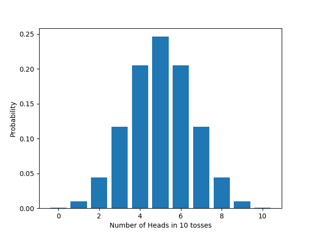
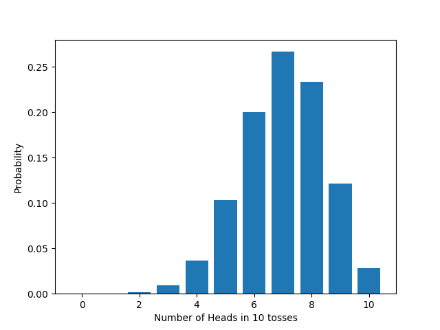
Here’s what the distribution looks like, in numbers, for a fair coin ($q=0.5$) flipped 10 times.
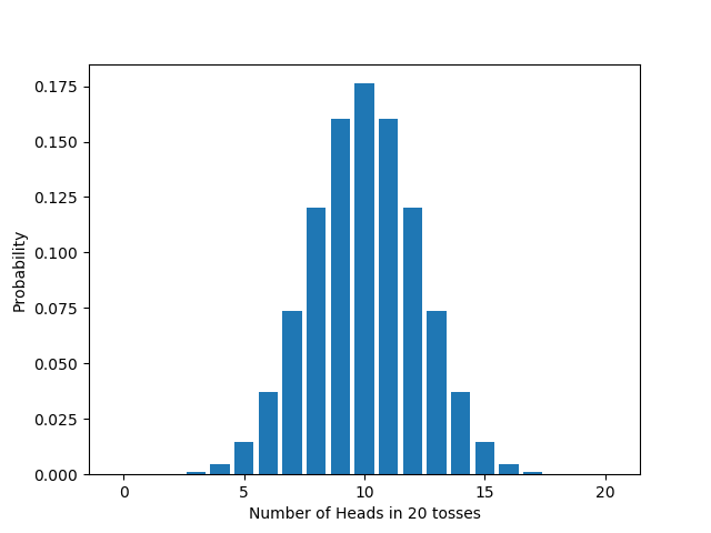
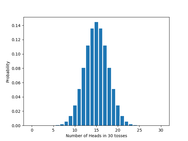
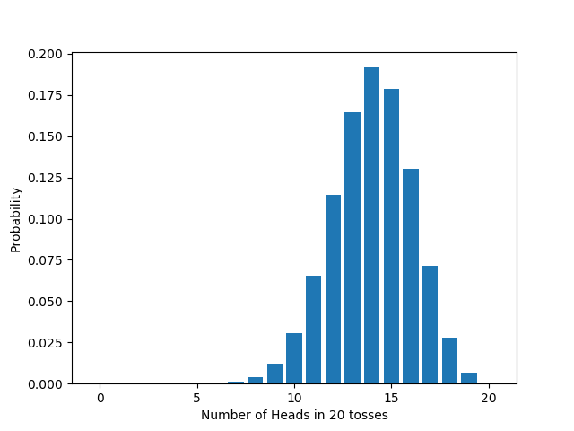
If we vary $n$, the number of times we flip the coin, the distribution changes too, in accord with the formula we derived above. For example:
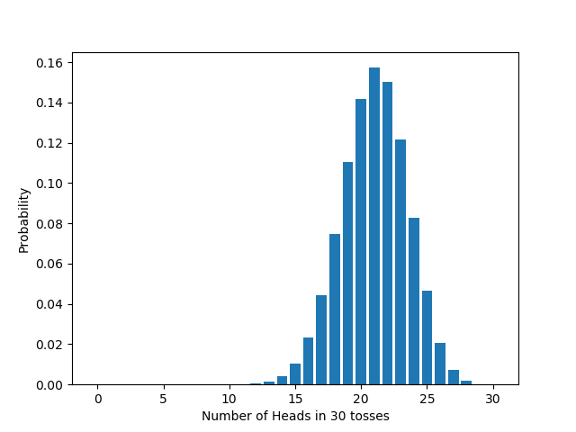
And if we take a biased coin ($q=0.7$), again the distribution changes, in accord with the formula above. For example:
How significance tests work
A significance test is a method of evaluating a probabilistic hypothesis. How do significance tests work? The procedure itself is quite simple, but the motivation for the procedure is subtle. So let’s build up to it in stages, to understand why it works the way it does.
Building up to a significance test
Remember the coin you modified earlier. We want to evaluate the hypothesis that the coin is fair. Suppose we flip it some number of times, and see that there are many more heads than tails. Does this give us reason to think it’s biased?
This is a tricky question because, as pointed out earlier, a fair coin can produce any outcome—and so can a biased coin (as long as there’s some non-zero chance of it landing heads and tails). In other words, if you flip your coin repeatedly and look at the resulting sequence, you can’t tell for sure whether your coin is fair or biased. To take an extreme case: it’s possible to flip a fair coin 1000 times and get heads every time. That’s the nature of chance.
Still, even though your coin—fair or biased—can produce any outcome, some outcomes are more likely than others, depending on the bias of the coin. Take the extreme case above: the probability of flipping a fair coin 1000 times and getting heads every time is $0.5^{1000}$. That’s small. In decimals, it’s about
So if we flip a coin 1000 times and get heads every single time, we might think that the sheer improbability of getting this sequence for a fair coin gives us very good reason to think that the coin isn’t fair. In other words, we might think that if our result is very improbable on the assumption that the coin is fair, we should reject that assumption.
But wait a second. There’s a big problem with this line of thought. Suppose your coin is fair, and suppose you flip it 1000 times and get not a sequence of 1000 heads, but some other sequence of heads and tails, say:
What’s the probability of getting this sequence, assuming the coin is fair? Well, it’s $0.5^{1000}$—exactly the same as the chance of getting 1000 heads. A fair coin has an equal chance of getting any particular sequence—the chance of getting any one of them is extraordinarily tiny. But surely not every outcome gives us reason to think the coin is biased.
So the reasoning we just went through can’t be right. We need something stronger than just the claim that our particular result was improbable. But we can modify the reasoning in a way that gets around this worry, by looking not at the result itself, but at properties of the result. We can pick a characteristic of the result—a test statistic—and see how improbable it is to get a result like the one we got, insofar as the test statistic is concerned. Note that this involves a human decision: by picking a test statistic, we’re deciding what to look at when we group results together as “alike”; the numbers aren’t making that decision for us.
For example, we can pick the number of heads as our test statistic. Instead of asking how unlikely it is, assuming the coin is fair, to get the particular sequence of flips we got, we can instead ask how unlikely it is, assuming the coin is fair, to get the number of heads we got. Suppose, for example, that there are 511 heads in the sequence above. The probability, assuming the coin is fair, of getting that many heads, is:
$${1000 \choose 511} \frac{1}{2^{1000}}$$
which is 0.01980746048584404.
This goes a long way toward fixing the problem above. A long way, but not all the way, for notice that it’s still very improbable that we get exactly 511 heads—and similarly for any other number of heads. So getting an improbable number of heads can’t by itself be a reason to think the coin is biased.
So we pull one more trick, and ask not whether it was unlikely, assuming the coin is fair, that we get exactly that many heads, but whether it was unlikely, assuming the coin is fair, that we get that many heads, or a more extreme result.
What does “more extreme” mean? There are two obvious ways to go here. One is to say: that many heads, or more; this is called a one-tailed test. The other is to say: that many heads or more, or that many tails or more (in other words, at least as far away from the expected number); this is called a two-tailed test. Which one of these we pick, like which test statistic we pick, is largely a matter of convention. But once we make that decision, we can calculate the chance that a fair coin would give us a result as or more extreme with respect to our test statistic; this is what’s called the $p$-value.
This gives us the traditional significance test, originally formulated by Ronald Fisher: a result gives us reason to reject our hypothesis if its $p$-value is small enough, given some (conventional) choice of test statistic, one- or two-tailed test, and value for “small enough” (called the “size” or “significance level”).
Looking at $p$-values graphically
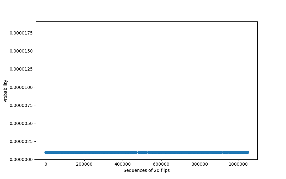
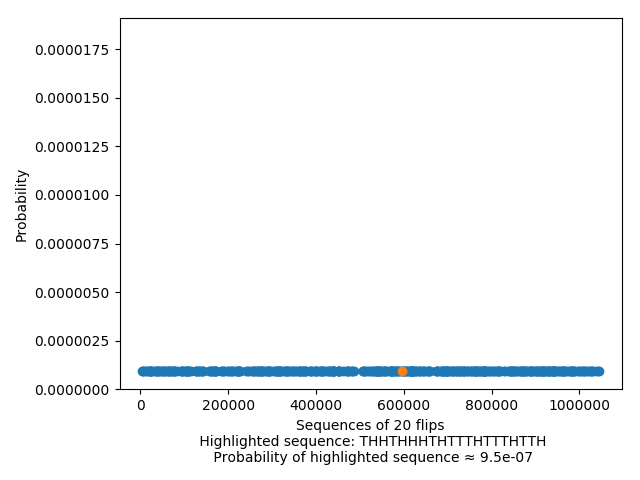
We can put the above reasoning graphically. If we graph the probability of getting any particular sequence, we get a flat distribution if the coin is fair, since each sequence is equally (un)likely:
And looking at the chance of any one sequence is just looking at the (tiny, tiny) value of any one of these points:
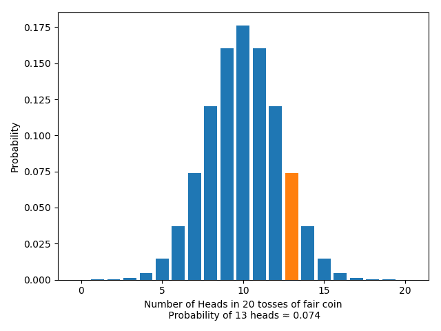
On the other hand, if we look at the distribution of the chosen test statistic, the number of heads, we get the binomial distribution we derived above:
Looking at the likelihood of the test statistic itself amounts to just looking at the likelihood of getting some particular number $m$ of heads:
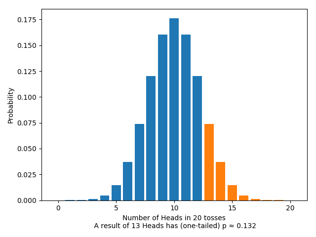
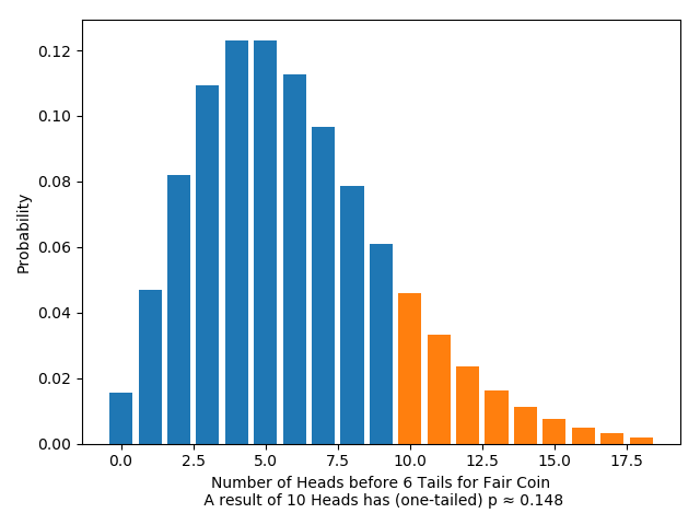
On the other hand, looking at the $p$-value means looking at the likelihood of getting any result as or more extreme than $m$ heads: rather than one single result, we’re looking at the area of an entire region. For the one-tailed test, this looks like:
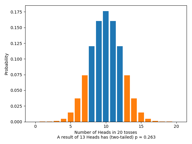
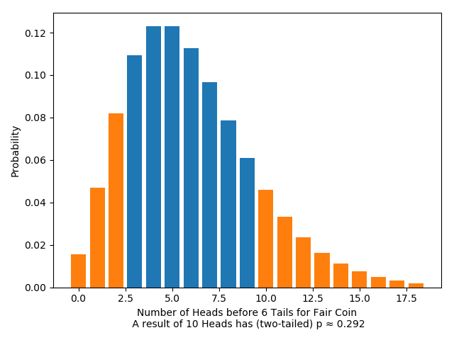
And for the two-tailed test, this looks like:
The General Procedure: A Warning
Let’s go over the driving idea behind the test. We want to test whether your coin is fair. Assume for a moment that it is fair. Then if we flip it 20 times, we expect to get about 10 heads. Suppose we actually get 8 heads. That’s not surprising, given our assumption. After all, we only expected to get about 10 heads, not exactly 10 heads. So the result doesn’t call our assumption into question. Suppose instead we actually get 4 heads. To get a result that far from 10 is surprising, given our assumption. So the result does call our assumption into question: either a surprising thing happened or our assumption is wrong. Now, surprising things do happen, but they don’t happen that often, else they wouldn’t be surprising. So the better bet is to reject the hypothesis that the coin is fair. That’s the idea behind significance tests.
In general, suppose we wish to test some probabilistic hypothesis, designated the null hypothesis. Design an experiment and determine all possible experimental outcomes. Then choose a test statistic, which associates a number with each outcome. Assuming that the null hypothesis is true, work out the distribution of the test statistic: that is, for each possible value of the test statistic, work out the probability of getting that value. Next, choose a significance level $\alpha$, typically 0.05 or 0.01, and decide whether to do a one-tailed or two-tailed test. Then do the experiment and note the actual value of the test statistic. Work out the the $p$-value. If the $p$-value is less than $\alpha$, reject the null; else, don’t.
Life would be much easier if the $p$-value of an experiment were the probability that the null hypothesis is true. But it’s not. The truth is more of a mouthful: the $p$-value is the probability of getting a value for the test statistic at least as extreme as the actual value, assuming the null is true. That is quite different to the probability that the null is true.
A lot of technical work has gone into developing significance tests. For example: working out the distribution of a test statistic can be hard and require some sophisticated math; extending the tests to cases where the data is continuous requires further machinery. But the driving idea behind significance tests is simple: do an experiment, and check how extreme the result is, assuming the null.
A different experiment
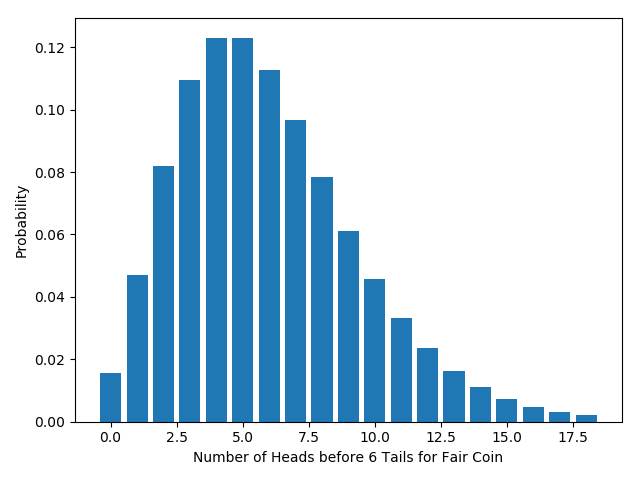
Suppose we had done our experiment differently: instead of flipping a fixed number of times, we decide we’ll keep flipping until we get a total of 6 tails. This is a perfectly sensible test, because we expect different behaviors from a biased coin and a fair coin: we’d expect a fair coin to take around 12 flips to get 6 tails, a tails-biased coin to do so in fewer flips, and a heads-biased coin to take a longer number of flips. We can even keep the same test statistic: the number of heads will vary between runs, since the length of runs will vary, and the number of heads is always 6 less than the number of flips. We expect around 6 heads for a fair coin. But in this setup, the distribution of the test statistic is different.
What is the distribution? We can work this out from the principles above. Assume the coin has a probability $q$ of getting heads on each flip. If a complete run of our experiments results in $m$ heads, we must have flipped it $m+6$ times, with tails on the final flip. In other words, we get a total of $m$ heads if and only if we got $m$ heads in the first $m+5$ flips, and then a tail. The chance of getting $m$ heads in the first $m+5$ flips is given by the binomial distribution we derived early on: ${m+5 \choose m} (1-q)^5 q^m$. The chance of getting a tail on the final flip is just $1-q$. So the total probability of getting $m$ heads is just ${m+5 \choose m}q^m (1-q)^6$. More generally, the total probability of getting $m$ heads by the time we get $r$ tails is ${m+r -1 \choose m} q^m (1-q)^r.$
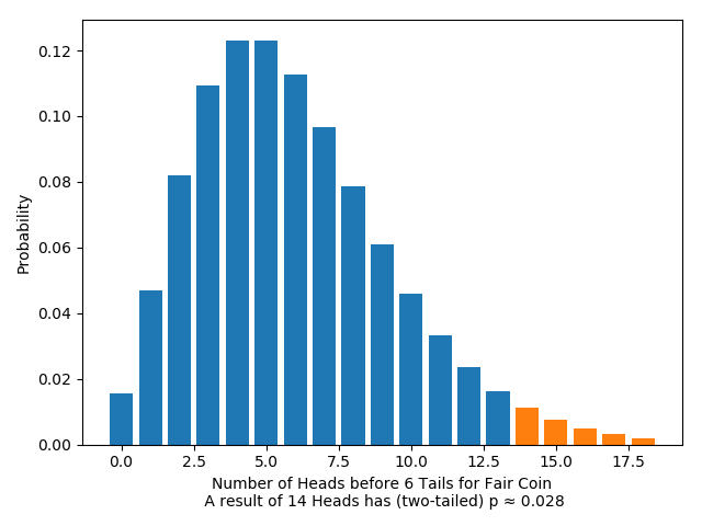
Again, this distribution has a special name: the “negative binomial distribution”. If we graph this distribution for a fair coin ($q=0.5$), it looks like this:
As before, we can calculate the $p$-values (one- and two-tailed) for any given result. For example:
Significance tests are sensitive to the stopping rule
We can express the difference between the two experiments as a difference in when we agree to stop the experiment. In the fixed-number-of-flips experiment, we stop when and only when we reach our target number of flips. In the fixed-number-of-tails experiment, we stop when and only when we reach our target number of tails. In other words, the two experiments have different stopping rules. (Of course, innumerably many other stopping rules are possible too.)
Suppose we perform both experiments: in the fixed-flips experiment we decide to flip a total of 20 times; in the fixed-tails experiment, we decide to flip until we get 6 tails.
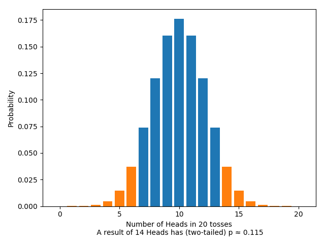
Some outcomes are possible in your experiment but not mine, such as a sequence of 9 h‘s and 11 t‘s; other outcomes are possible in mine but not yours, such as a sequence of 8 h‘s and 6 t‘s, ending in a t; but some outcomes are possible in both our experiments, such as hhhththhhhhthhthhhtt, a total of 6 tails, 14 heads.
Let’s do significance tests on the two experiments. As far as our choices of conventions, we’ll pick the same conventions for both: both will test the null hypothesis that the coin is fair; both will use the number of heads as a test statistic; both will use a two-sided test; both will reject the null hypothesis only if the $p$-value is less than $0.05$ (a typical choice). Let’s suppose that, as it happens, we get the same outcome in both experiments, the one at the end of the previous paragraph.
Pulling from the above, for the fixed-flips test we have:
The $p$-value here is greater than $0.05$: according to the test, it’s not a result significant enough to warrant rejecting the null hypothesis that the coin is fair.
At the same time, for the fixed-tails test, we have:
The $p$-value here is less than $0.05$; according to the significance test, this is a result that is significant enough to warrant rejecting the null hypothesis.
But the only difference between the two situations is the stopping rule used! In other words, the very same sequence of coin flips, with the very same conventions, leads to opposite conclusions, depending on which stopping rule was used. That’s what we mean when we say that significance tests are sensitive to the stopping rule.
Is sensitivity to the stopping rule a problem for significance testing?
Plenty of other objections have been leveled at significance tests. But sensitivity to the stopping rule is at the heart of the dispute. Take Deborah Mayo, for example, a staunch defender of significance tests: “Edwards, Lindman, and Savage, quite rightly, regard this difference in attitude on the relevance of stopping rules as a central point of incompatibility between [rival methodologies in statistics].” (Mayo, 1996: 342) Howson and Urbach agree on the centrality of stopping rule sensitivity, although they disagree with Mayo about what conclusion we should draw from it: “The fact that significance tests [are sensitive to the stopping rule] is a decisive objection to the whole approach.” (Howson and Urbach, 2006: 159)
So, then, is sensitivity to the stopping rule a problem for significance testing or not? Examples involving coins can make the question seem academic. Far from it: if stopping rule sensitivity is a problem, we need to know. The question isn’t academic, and nor is it easy. The rest of the post sketches some of the arguments, pro and con. The parts can be read in any order. About half of what I write below is false. But which half?
Irrelevance.
ExpandClose
Suppose you do the fixed-flips test and I do the fixed-tails experiment. If someone watches footage of our two experiments, what will she see? She’ll see you flip a coin repeatedly and end up with the sequence hhhththhhhhthhthhhtt; and she’ll see me flip a coin repeatedly and end up with the same sequence. Of course, you intended to flip it 20 times and I intended to flip it until I get a total of 6 tails. But our intentions don’t show up on screen. From our observer’s point of view, our experiments are indistinguishable—until the end, when she’ll see me reject the null and you not.
$$$$
Fix an hypothesis $H$ and data $D$. Either $D$ is evidence against $H$ or it’s not. In our example, $H$ is that the coin is fair and $D$ is the sequence of coin flips. In my test, $D$ is taken to be evidence against $H$. In your test, it’s not. So one of the tests goes wrong. More generally, whenever a significance test yields one verdict under one stopping rule and another under another, one of the verdicts will be wrong. Therefore, absent any advice about which stopping rules to use, significance tests should not be relied on.
$$$$
Compare: Suppose I propose a method for evaluating probabilistic hypotheses. The method has a curious property: it’s sensitive to the weather. If it’s raining, a particular experimental outcome is taken to *refute* some hypothesis; if it’s sunny, that same experimental outcome is taken *not* to refute it. Obviously, that’s a vice: no method should be sensitive to the weather. But sensitivity to the stopping rule is no better. No method should be sensitive to anything other than the experimental outcome: same outcome, same inference.
Cheating
ExpandClose
Suppose you are an unscrupulous scientist, seeking reason to reject some rival scientist’s hypothesis. Perhaps you can exploit sensitivity to the stopping rule: do a significance test, choosing your stopping rule carefully so as to boost the probability of rejecting the hypothesis.
$$$$
Take your coin. Suppose I offer a prize if you manage to bias it; I’ll award you the prize if a two-tailed significance test, with test statistic the number of heads, rejects the hypothesis that the coin is fair at a significance level of 5%. You could just do a fixed-flips test, flipping it 20 times, say. But how might you exploit sensitivity to the stopping rule to boost your chances of rejecting the null and winning the prize?
$$$$
Here’s one attempt: flip the coin until you have 10 more heads than tails. Actually, let’s add a cut-off: flip the coin until you have 10 more heads than tails *or* you’ve flipped it a total of 100 times, whichever comes first. (Adding the cut-off simplifies the analysis; but we could make the same point even if we dropped it.) Call this the *fixed-difference* stopping rule. By choosing the fixed-difference rule, you’ve considerably boosted the probability that you’ll get 10 more heads than tails. So haven’t you also boosted your chances of rejecting the null?
$$$$
Let’s work it through. First, take the fixed-flips test. When will we reject the null? Well, if we observe no heads at all, we’ll get a *tiny* $p$-value ($2 \cdot \frac{1}{2^{20}}$), so reject. If we observe 1 head, we’ll get a slightly bigger, but still tiny, $p$-value, and still reject. Calculating $p$-values in turn for each possible number of heads, it turns out we reject if the number of heads is between 0 and 5 or 15 and 20, inclusive. So the probability that we reject is the probability that we get between 0 and 5 heads or 15 and 20 heads, inclusive. Assuming the null is true, that’s about 4.1%.
$$$$
What about the fixed-difference test? This is more complicated. In the fixed-flips test, we can get any number of heads from 0 to 20; but in the fixed-difference test, we can get any number of heads from 0 to 55. (Exercise: Why can’t we get more than 55 heads?) To derive the distribution takes some work (if you’re interested, google “simple random walk”), but here’s the graph:
When will we reject the null? Calculating $p$-values in turn for each possible number of heads, as before, it turns out we reject if the number of heads is between 0 and 17, inclusive. So the *probability* that we reject is the *probability* that we get between 0 and 17 heads, inclusive. Assuming the null is true, that’s about 4.3%.
$$$$
So, admittedly, with the fixed-difference rule we have a slightly higher chance of rejection than with the fixed-flips rule. But the difference is small (4.3% v. 4.1%). That sort of fluctuation isn’t surprising. For example, the chance of rejection in a fixed-flips test where you flip it 20 times is slightly different to the chance of rejection in a fixed-flips test where you flip it 30 times, which is slightly different again to the chance of rejection in a fixed-flips test where you flip it 40 times. Whenever you change your stopping rule, a small fluctuation in the chance of rejection is to be expected. The key point is that when you moved from fixed-flips to fixed-difference, the chance of rejection was pretty much the same; you certainly didn’t significantly boost your chance of rejecting the null, as you hoped.
$$$$
There’s no deep mystery here. When we moved from fixed-flips to fixed-difference, we *did* boost the chance of observing 10 more heads than tails; in the fixed-flips test, observing 10 more heads than tails (i.e. 15 heads and 5 tails) leads us to reject the null. *but in the fixed-difference test, it doesn’t.* Why not? Because changing the stopping rule also changes the distribution of the test statistic, and so changes which values for the test statistic lead to rejection. What you’ve gained on the swings, you’ve lost on the roundabouts. In fact, it’s straightforward to show that in any significance test, the chance of rejection, assuming the null, is at most the significance level. Change the stopping rule however you like, you won’t boost the chance of rejection above 5%.
Rarity
ExpandClose
Even if sensitivity to the stopping rule is a problem, doesn’t it show up only rarely? After all, in our coin example, it’s unlikely that you and I will get the same outcome, so it’s unlikely that the sensitivity to the stopping rule will actually come up in practice.
$$$$
Agreed: it’s unlikely that you and I will get the same outcome in the coin example. But our two stopping rules do not exhaust the possibilities. The space of possible stopping rules is large. Given that, surely for almost all outcomes in almost all experiments, there are stopping rules such that one leads to rejection and the other doesn’t.
Probability of false rejection
ExpandClose
Imagine a machine that plays Tetris. The machine plays well. In fact, the engineer provides a performance guarantee. Since Tetris has a random element—the order and orientation of the falling blocks—the engineer can’t guarantee that the machine *always* gets a score over 100. It might be unlucky. But the engineer can provide a *probabilistic* performance guarantee: with probability 95%, the machine gets a score over 100.
$$$$
After a while, you notice a strange fact: a copy of the machine in Cambridge and a copy of the machine in Oxford play simultaneously, and by chance the blocks in the two games fall in the same order and orientation. But the machines behave differently. It ends up that the machine in Cambridge gets a score over 100 but the machine in Oxford gets a score less than 100. When you inspect the code, it turns out that the behavior of the machine is sensitive to something surprising: whether it’s raining where the machine is. If it is raining, the machine behaves one way; if it’s not, the machine behaves another. Still, the engineer’s performance guarantee is true: if it’s raining, the machine gets a score over 100 with probability 95%; similarly if it’s not raining; so similarly overall.
$$$$
Significance tests, so the thought goes, are like the Tetris machine. They also come with a probabilistic performance guarantee: if you do a significance test with significance level 5%, then with probability 95% you won’t reject the null when it’s true. That is a virtue of significance tests: the probability of mistakenly rejecting the null is low. Just as the Tetris machine is sensitive to the weather, so too the significance test is sensitive to the stopping rule. But in neither case does that sensitivity undermine the performance guarantee. No matter the stopping rule, the probability of mistakenly rejecting the null is low. Isn’t that recommendation enough?
Relevance
ExpandClose
Suppose you have two experiments: in the first, the experimenter flips the coin until he gets more heads than tails; in the second, the experimenter flips the coin 101 times. Both get the same outcome—the very same sequence of h‘s and t‘s. The outcome contains 51 heads and 50 tails and the number of heads exceeds the number of tails only on the last flip. Surely the outcome points in different directions in the two cases. In the first case, you should be more confident than not that the coin is tails-biased. (After all, it took a long time—101 flips—to get more heads than tails.) In the second case, you should be more confident than not that the coin is heads-biased. (After all, there are more heads than tails.) Which way the experimental outcome points depends on the stopping rule. Therefore being sensitive to the stopping rule is a virtue, not a vice.
Stopping rules in practice
ExpandClose
Remember the coin example: your stopping rule is to flip it 20 times; mine is to flip it until I get a total of 6 tails. Your stopping rule is perfectly natural; but mine is odd, and isn’t the kind of thing used in practice. Perhaps the stopping rule sensitivity only arises when we bring in these odd stopping rules. Given the stopping rules used in practice, the phenomenon doesn’t arise, so can be safely ignored.
$$$$
Well, maybe. But it’s not at all obvious that stopping rule sensitivity does only arise with ‘odd’ stopping rules. Besides, even if it’s true, it may not be enough. Perhaps the fact that significance tests are sensitive to stopping rules at all shows that there is something wrong with the methodology. To rest easy just because the phenomenon doesn’t come up in practice is to confuse suppressing a symptom with curing the disease.
If you don’t look up, Dynamicland seems like a normal room on the second floor of an ordinary building in downtown Oakland. There are tables and chairs, couches and carpets, scattered office supplies, and pictures taped up on the walls. It’s a homey space that feels more like a lower school classroom than a coworking environment. But Dynamicland is not a normal room. Dynamicland was designed to be anything but normal.
Led by the famous interface designer Bret Victor, Dynamicland is the offshoot of HARC (Human Advancement Research Community), most recently part of YCombinator Research. Dynamicland seems like the unlikeliest vision for the future of computers anyone could have expected.
Let’s take a look. Grab one of the scattered pieces of paper in the space. Any will do as long as it has those big colorful dots in the corners. Don’t pay too much attention to those dots. You may recognize the writing on the paper as computer code. It’s a strange juxtaposition: virtual computer code on physical paper. But there it is, in your hands. Go ahead and put the paper down on one of the tables. Any surface will do.
Photo by by Alex Handy
Now you see this is not a normal room at all. Suddenly there’s something else on the table. Something dynamic and visual. It may even be making a sound. Grab some more of those pieces of paper. Slap them down on the table as well. Shapes, characters, and noises are now inhabiting this room alongside you. They grow, move, and distort along the table, interacting with each other, and possibly with physical objects on the table, like popsicle sticks, colored cubes, and small robots on wheels.
Yet it’s still just a room. Not virtual reality. Not augmented reality. Certainly not blockchain-reality. It’s a mostly normal room. That is until you get it started. Or look up.
Now you look up. The ceiling is quite full. There suspended are dozens of high-powered projectors, cameras, and speakers, all pointed down at the room, waiting for your code to make them come alive.
Dynamicland is a new kind of computer. It’s not a gadget that you keep in your pocket, nor one you can slip into your bag. The whole darn room is the computer.
Illustration by Dynamicland
A computer the size of a room? No screens? What antiquated notions! This vision looks very different than the virtual reality we’re eagerly anticipating.
Tye Sheridan in Ready Player One. Credit to: Warner Bros.
The better our computers and smartphones get, the further we get from physical reality, and the more we want to leave it behind entirely. We are tired of our limiting bodies holding us back with their aching backs, bleary eyes, and strained finger joints. As Victor says:
We’ve almost given up on the body already. We sit at a desk while working, and sit on a couch while playing, and even sit while transporting ourselves between the two. We’ve had to invent this peculiar concept of artificial “exercise” to keep our bodies from atrophying altogether.
It won’t be long before almost every one of our daily activities is mediated by a “computer” of some sort. If these computers are not part of the physical environment, if they bypass the body, then we’ve just created a future where people can and will spend their lives completely immobile.
Why do you want this future? Why would this be a good thing?
In The Human Representation of Thought, Bret Victor pointed to this picture of the ascent and descent of man, “This is what it means to do knowledge work nowadays. This is what it means to be a thinker. It means sitting and working with symbols on a tiny rectangle… This style of knowledge work, this lifestyle is inhumane.”
Our computers have lured us into a cage of our own making. We’ve reduced ourselves to disembodied minds, strained eyes, and twitching, clicking, typing fingertips. Gone are our arms and legs, back, torsos, feet, toes, noses, mouths, palms, and ears. When we are doing our jobs, our vaunted knowledge work, we are a sliver of ourselves. The rest of us hangs on uselessly until we leave the office and go home.
Worse than pulling us away from our bodies, our devices have ripped us from each other. Where are our eyes when we speak with our friends, walk down the street, lay in bed, drive our cars? We know where they should be, and yet we also know where they end up much of the time. The tiny rectangles in our pockets have grabbed our attention almost completely.
And worst of all, we’ve lost sight of the most salient part about computers: their malleability. We’ve acquiesced the creation of our virtual worlds, where we now spend most of our time, to the select few who can spend the millions to hire enough software engineers. So many of the photons that hit our eyes come from purely fungible pixels, yet for most of us, these pixels are all but carved in stone. Smartphone apps, like the kitchen appliances before them, are polished, single-purposes tools with only the meanest amount of customizability and interoperability. They are monstrosities of code, millions of lines, that only an army of programers could hope to tame. As soon as they can swipe, our children are given magical rectangles that for all their lives will be as inscrutable as if they were truly magic.
In many respects, Alan Kay, co-founder of Dynamicland and “intellectual parent” to Bret, is largely responsible how our computers look and work today. Infamously in 1979, Steve Job visited Xerox PARC and later used many of Kay’s ideas in the Apple Macintosh (which in turn were used in the Windows operating system). Less well known is that in 1975 Kay proposed a computational tablet, the “Dynabook”, that bears much resemblance to the modern iPad!
One way to understand Dynamicland is as a reaction to the wild success of, and the subsequent regrets about, Xerox PARC. The original inventors of computers didn’t mean to be taken so literally. This was just one possible vision for computing–not the only one and certainly not the best one. Today Bret is showing us a better way forward. A more humane computer. And that computer is not a device. It’s a normal-seeming room.
We shouldn’t be that surprised. Almost every room in every building is also normal-seeming, but quietly powered with technology embedded in the ceiling. Light! It’s so commonplace now that we hardly spare it a thought. Every room comes equipped with one or more buttons in the wall to control these lights. We’ve made on-demand lighting a part of our infrastructure.
Light is not a device we charge up and carry around in our pockets. Imagine how much dimmer that world would be: people carrying flashlights, shooting small cones of light wherever they go. It would be a small, lonely, personal world, a world where we only get to see one thing at a time, a world where one of your hands is always full with an electronic gadget.
That’s what Dynamicland is trying to show us: we do live in that atomized, handheld world. We charge up and carry around our personal computing devices for our eyes only. New technology is eagerly anticipated as something to wait in line at the Apple Store for, to be purchased and coveted, not invested in and shared as a public utility.
When you invest in public utilities, like roads, electricity, light, you get more than you pay for. You get so many things “for free.” This is also the case at Dynamicland. There are many, many things that come “for free” as a function of its design.
For one, you get “multiplayer”, Google-docs-style collaboration for free. At Dynamicland computing is social like cooking is social. It’s also physical like cooking is physical. You’re not seated in front of a single-person screen, but walking around an open space, using a range of tools. It’s incredibly natural to walk up to someone “cooking” up some code, offering to lend a hand, divvying up tasks, and improvising on the fly. You use your hands in all the myriad ways they’re meant to be used:
Photo by Bret Victor
When I visited Dynamicland in January, I was building on a spreadsheet-like program next to my friend Omar who was building a map-based interface. Just by virtue of sitting next to each other, we were able to keep apprised of what the other was up to. At some point Omar needed a way to input a number to control the zoom of his map. My spreadsheet program had plenty of numbers, and ways to manipulate numbers, so we slid over one of my pieces of paper and it immediately worked to zoom into his maps. Omar decided that he’d prefer a slider-based number-input, and after it was built, he slid it over to my side of the table, and we used a multiplication operator I had built to expand the slider’s range. Again, it just worked. At Dynamicland you get composability and interoperability “for free.”
Much of what you get “for free” at Dynamicland comes from the fact that it’s embedded in a very powerful computation engine: reality. The world is naturally built for multiple people. The world also has many contrivances for inputting data: buttons, pages, layouts, and drag-and-drop. At Dynamicland, there’s no need to code any of that. We can outsource that computation to its original source and merely capture it via cameras on the ceiling. The slider Omar built was a pebble on top of a long strip of paper. The numbers I made were square pieces of paper that you could place colored “poker chips” onto, each color chip representing different multiple of ten. Anywhere a number is required, either will do — or any other number representation you dream up and program into the system. Copy-and-paste is literally making a photocopy and literally pasting something with glue or tape where you want it. Drag-and-drop is, well, physically moving objects around. The user interface phrases “direct manipulation” and “what you see is what you get” (WYSIWYG) have quite literal meanings at Dynamicland.
Dynamicland is designed to be understandable, modifiable by all. There’s almost a Jeffersonian spirit of rustic individualism about the space. Code is always shown in plain view, printed right on each page. Moreover, it’s considered “bad style” to write code that fits on more than an 11×17 sized page of printer paper. The whole system, Realtalk OS, runs on mere thousands of lines of code, two whiteboards, back to back. That’s it.
Realtalk OS by Bret Victor
It’s understandability, customizability, and mashup-ability by default — a stark contrast to the slick, polished, and discrete apps on our home screens. Instead of apps, people build “kits”, aggregations of various pages that augment each other. My friend Omar has spent a lot of time putting together Geokit, which allows you to print out maps, move them around, zoom in and out, and layer on demographic data. But it’s just a kit, a few pieces of paper in a box. You can use it in conjunction with other little paper programs you’ve created, other kits, or get your hands dirty by modify its code directly. If the changes you’ve made are good, grab the “Print this page” page and point it at your modified code. The new version is waiting for you at the nearest printer.
Geokit’s parts by Omar Rizwan
This kind of fluid, flexible media could entirely reshape children’s relationship with technology. Instead playing Flappy Bird, Minecraft or Fortnite, imagine kids co-creating a hybrid digital and physical game together. Make-believe meets the digital age.
From the Dynamicland Zine
It’s also not difficult to imagine a future Dyanmicland-inspired living room where a family could invent a new game like Laser Socks in a couple hours and play it that same night!
Laser Socks by Glen Chiaccchieri
The printing press was perhaps the greatest time technology gave us the tools to understand the world around us. The mass-printed word gave us revolution in every corner of humanity: religious with Martin Luther’s Ninety-five Theses; political with Locke, Paine, and newspapers; scientific with Newton, Galileo, and research journals; and artistic with the birth of the novel. As a society we decided that this new medium deserved to be in the hands of the people, elevating and enlightening us all. It was a requirement of democracy to have a free press and well-read public. That’s why we built our libraries: normal-seeming rooms, open to the public, and packed to the brink with all of the knowledge of humanity’s best thinkers through the ages.
If you walk into a library today, these once proud books mostly sit and collect dust. Occasionally someone will check one out, but physical books no longer have the allure they once had. They can be gotten easier and quicker – albeit still not cheaper – via our digital screens. But libraries still have their uses. If you duck around the stacks of books and head to the back, you’ll see a diverse crowd filling up almost all of the seats. Most of them are on their computers, some are on the computers provided by the library, and a few are reading books. Isn’t it a bit sad that in this beautifully public space, everyone is off in their own world, doing their own thing? There’s no talking. There’s no collaboration.
What if we decided to reimagine our public intellectual spaces to fit the new medium of the day? What if we built our public spaces to be truly public, truly shared, and reverse some of the atomizing influences of the last media revolution?
Libraries didn’t happen by accident. Andrew Carnegie built 2,509 of them with his own money. Dynamicland isn’t cheap, and it too won’t happen by accident. It’s scraping by with just enough funding each day. Will a modern-day Carnegie come to its, and all of our, rescue? Or will we need to take matters into our own hands, making a thousand small little donations on the Dynamicland website? Or could it be possible that the government foots the bill on this one? Or most likely yet, will Dynamicland fade into the background as one more vision of the future that never comes to pass? What future do you wish to inhabit? Think on these questions the next time you walk into a room and flip on the lights.
Phenomenal World is a new publication that publishes research, analysis, and commentary on applied social science. We chose this name for our blog because we hope to publish work that addresses the social world in all its apparent complexity.
Our contributors are economists, philosophers, social scientists, data scientists, and policy researchers. You’ll find posts on metaresearch; basic income, welfare and the commonwealth; digital ethics; education; economic history; and evolving institutions. We also post our weekly newsletter, a roundup of recommended reading from across the social sciences. Posts are wide-ranging in subject matter, length, and style.
Phenomenal World is managed by staff of the Jain Family Institute, an applied research organization that works to bring just research and policy from theoretical conception to actual implementation in society. We welcome submissions. Please see our About page for more information on submitting, and for the sign-up form for our newsletter.
 World