Comments Off on Decision Making in a Dynamic World
I once wrote a post criticizing modern microeconomic models as both overly complex and unrealistic, leading their practitioners into theoretical dead ends without much corresponding increase in explanatory power. I suggested the entire enterprise of Expected Utility (EU) was a dead end based on a mistake and that I’d eventually write about superior ways of modelling individual decision making under uncertainty. It’s been a long time coming, but below I outline why taking time into account leads to better theories of decision making, and why human psychology does a fairly good job of guiding decisions in a dynamic world.
The Poverty of EU-style Theories
I see EU as an attempt to transpose the mathematical world of probabilities onto the real world of making decisions. It was originally theorized that people make decisions based on the simple Expected Value (EV) of potential outcomes: that is, that they weigh the monetary value by the probability a given outcome will happen, and then add them all up. There was no empirical reason to believe this was an accurate description of how people made decisions, nor was there any scientific value in doing so. One of the earliest contradictions EV couldn’t resolve was the St. Petersberg paradox, introduced by Daniel Bernoulli in 1738: I flip a coin and pay you £2 if it comes up tails, but double the pay out and flip again if it comes up heads; then next time pay you £4 if it comes up tails, but double and flip again if it’s heads; and so on, forever. The EV of this gamble is infinite, so anyone reasoning according to EV would pay an infinite amount to take part in the game. Intuitively, we recognize that this behavior would be both irrational and impossible. Bernoulli proposed to settle the paradox by taking logarithms of the monetary outcomes—interpreted as diminishing satisfaction from increases in money—to make the outcome finite.
Ole Peters has spilled much ink over the limits of this solution. The crux of his argument is that EU treats the gamble as if it is done once for each person, but repeated for many different people, just like in a casino. If, instead, the individual thinks about their wealth over time, they will aim to maximize the growth rate of their wealth rather than the immediate amount, so a different type of calculation should be used. Mathematically this is equivalent to using the ‘geometric mean’ (timesing all the gambles together and rooting them by the number of periods) rather than the ‘arithmetic mean’ (adding all the weighted gambles together and dividing them by the number of periods). By using the former you arrive at a finite solution with no need to introduce any assumptions about the individual’s preferences over risk and money.
I agree with JasonSmith that Peters overstates his case by insisting that EU is a mathematical error; but we can still interpret Peters as arguing that EU theory is inapplicable and proposing a better alternative. Or as Wikipedia puts it: “the St. Petersburg paradox is only a paradox if one accepts the premise that rational actors seek to maximize their expected wealth.” There is no a priori reason to accept this premise, and it seems much more sensible to have a resolution in which individuals maximize their wealth over time—time being an important feature of the real world—and which otherwise makes fewer assumptions.
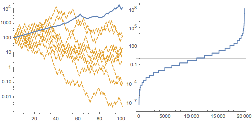
My friend Cameron Murray’s discussion of Peters provides a good example of why time is important here. Suppose you play a repeated game in which you start with £100, and if a coin flip comes up heads you win 50% of your current wealth, while if it’s tails you lose 40%. The majority of the time your outcome will not converge to the expectation as calculated by EV (blue line). In fact, you will generally lose money (orange lines):
People are intuitively aware of the possibility of going down a ‘bad’ path, which is why in many cases they use decision-making rules which try to avoid this, rather than anything resembling EU. One of the interesting side-effects of this is that not only do most people violate EU and time-consistency in experiments, but the violators actually earn more money! Living in a dynamic and changing world means that humans pursue flexible strategies to adapt to their environment. Thus, not only is EU empirically inaccurate; it is not a desirable standard for behavior.
Heuristics for the Real World
Peters’ contribution is a valuable first step toward dynamic decision theories, although it still rests on maximising behavior and so cannot form an accurate description of real decision making in general. Fortunately, a literature in psychology has taken to questioning the precepts of EU (including modern ‘behavioral’ variants such as prospect theory) and proposing theories more in line with what psychology tells us about human behavior under uncertainty. A significant contribution is the priority heuristic—proposed in a 2006 paper by Eduard Brandstätter, Gerd Gigerenzer, and Ralph Hertwig—which posits that, when faced with a choice of two gambles with two outcomes, people compare outcomes and probabilities separately and sequentially instead of weighting them all together.
To clarify, a ‘gamble’ in economics is typically a set of possible cash rewards, each with a probability. To start, the authors restrict themselves to gambles with two possible outcomes, and look at choices between different gambles. Gamble A could be a 50-50 chance of £5 or £15, whereas Gamble B could be a 10% chance of £50 or a 90% chance of £5. Economists, and to a lesser extent psychologists, have spent a great deal of time trying to predict which gamble people will choose in this type of problem.
Unlike EU theorists, the authors of the priority heuristic draw from an array of psychological literature to determine exactly how—in what order and using what criteria—people do this. They first conclude that there is a lot of evidence to suggest that people neglect probabilities, and are likely to consider outcomes first. They argue that ‘avoiding low minima’ is likely to be considered first because people are predisposed to avoid bad outcomes (see the simulations above). The next consideration is given to a probability, and based on a preliminary experiment the authors hypothesise that as with the outcomes, people will consider the probability of the minimum before that of the maximum. Once the probability of the minimum is known, the maximum is implicitly known so there is no need to include it separately. Thus the third and final consideration is given to the maximum outcome.
Finally, there is the question of how the outcomes and probabilities should be compared across gamblers. Not wanting to introduce a ‘degree of freedom’—a parameter we can manipulate to make our results fit better—the authors choose a rule based on the number 10, although they point out they would like to use an independently determined aspirations level in the future. We are left with the following procedure:
Priority rule: Go through reasons in the order: minimum gain, probability of minimum gain, maximum gain. Stopping rule: Stop examination if the minimum gains differ by 1/10 (or more) of the maximum gain; otherwise, stop examination if probabilities differ by 1/10 (or more) of the probability scale. [Beyond this, just compare the maxima directly] Decision rule: Choose the gamble with the more attractive gain (probability).
The priority heuristic is then tested across multiple experiments. In summarising its predictive power I cannot do much better than the abstract of the paper itself:
The priority heuristic predicts (i) Allais’ paradox, (ii) risk aversion for gains if probabilities are high, (iii) risk seeking for gains if probabilities are low (lottery tickets), (iv) risk aversion for losses if probabilities are low (buying insurance), (v) risk seeking for losses if probabilities are high, (vi) certainty effect, (vii) possibility effect, and (viii) intransitivities. We test how accurately the heuristic predicts people’s choices, compared to previously proposed heuristics and three modifications of expected utility theory: security-potential/aspiration theory, transfer-of-attention-exchange model, and cumulative prospect theory.
This is an impressive list of predictions which excludes some further advancements made by the decision strategy. Firstly, the heuristic correctly predicts the relative time taken by individuals to make decisions. If they are able to decide based on the minimum outcome, they will spend less time on the decision; if they have to go all the way to the maximum outcome, they will spend more time. Such are the benefits of a more descriptively accurate theory of behavior.
Secondly, in the few (13%) cases where the heuristic is an inferior predictor, it was because there were large differences in Expected Values between gambles. In these cases, simple EV does at least as well as EU or any behavioral theory, which implies simplicity is key to understanding decisions. Thirdly, the priority heuristic is still highly predictive when applied to gambles with more than two outcomes, suggesting that maxima and minima are especially salient for decision makers—a kind of bounding approach that is consistent with people wanting to make sure their decisions are much more likely to produce an upside than a downside.
It is a shame that this theory has not gained more traction in economics given its inherent plausibility and its empirical success, even in this basic form. It would be good to see some more systematic studies of how well EU-followers fare, both in experiments and outside them, including reviewing existing economics experiments where possible. It would also be good to see extensions of the priority heuristic to field settings. Nevertheless, both Peters’ paper and the psychology literature acknowledge much more clearly the role of time and the importance of avoiding a bad path in the change in wealth. While I find it implausible people maximise anything, one way of modifying Peters’ framework might be to look at salient wealth paths based on the kind of criteria used by the priority heuristic and choosing between them. In any case, there’s no excuse for clinging to unrealistic theories when we have such compelling alternatives.
As national and regional governments form expert commissions to regulate “automated decision-making,” a new corporate-sponsored field of research proposes to formalize the elusive ideal of “fairness” as a mathematical property of algorithms and their outputs. Computer scientists, economists, lawyers, lobbyists, and policy reformers wish to hammer out, in advance or in place of regulation, algorithmic redefinitions of “fairness” and such legal categories as “discrimination,” “disparate impact,” and “equal opportunity.”)1 More recently, salutary critical voices, warning against the limits of such proposals, have proliferated both within and without the loosely networked field.2
But general aspirations to fair algorithms have a long history. In these notes, I recount some past attempts to answer questions of fairness through the use of algorithms. My purpose is not to be exhaustive or completist, but instead to suggest some major transformations in those attempts, pointing along the way to scholarship that has informed my account.
Fair algorithms since the seventeenth century
In a broad sense, “algorithmic fairness” may refer generally to any use of algorithms seeking to achieve fairness in the resolution of social disputes. “Algorithm” derives from the late medieval Latin “algorismus,” from the name of the Islamic mathematician Al-Khwārizmī, whose manuscripts in Arabic described the Indian system of arithmetic. The word’s meaning eventually developed into the technical definition employed in today’s computer science: “any well-defined computational procedure that takes some value, or set of values, as input and produces some value, or set of values, as output.”3
According to linguist Anna Wierzbicka, “fairness” may denote a set of “cultural assumptions” regarding “the regulation of [human] life effected by stated and unstated rules of interaction,” rules that most interactants see as “generally applicable” and “reasonable.” This meaning in modern English developed in tandem with Anglo-American political philosophy, and “can be seen as related to the post-Enlightenment move away from metaphysics and to the shift from an ethics based on religion to a ‘procedural morality’ and to an ethics based on ‘reason,’ ‘social cooperation,’ and ‘each participant’s rational advantage.’”4
In the broad sense opened up by these definitions, the idea of fairness-by-algorithm dates back at least to the seventeenth century. In the narrow sense produced in recent scholarship, algorithmic fairness is often understood to refer specifically to the algorithmic risk classification of people, involving some mathematical criterion of fairness as a complementary consideration or constraint to the usual optimization of utility. My notes below move roughly chronologically, from the broader idea to the narrower concept.
Since ancient times, moral theorists have formulated conceptions of justice on the basis of mathematical ideas. Aristotle discussed distributive and corrective justice in terms of geometrical and arithmetical proportion respectively.5 But it was only in the early modern period that more systematic efforts to use mathematical calculations to resolve political conflicts about justice and fairness emerged. For example, in seventeenth-century England, competing methods for calculating the “present value” of future property sought to answer a question of fairness: how much a piece of property to be exchanged in the future ought to be worth in the present. Historian William Deringer reports that as early as the 1620s, mathematicians developed “present value” tables for determining fair terms for certain agricultural leases, especially of land owned by the Church of England.6 In 1706, such mathematical calculations became relevant to a major political question: how to balance the terms of the potential constitutional union between England and Scotland. The debate centered on how to determine the fair value of a proposed monetary “Equivalent” that was to be paid up front by the English government to Scottish stakeholders in compensation for higher future tax rates. On the basis of a calculation of compound-interest discounting, the English agreed to pay £398,085 and 10 shillings.7 Multiple factors enabled this puzzling possibility of resolving an important political conflict through an elaborate mathematical calculation, including the persistent legacy of Aristotelian ethics and the weakening of the Church as an institution of public trust.
In the Enlightenment, ethical questions were central to the initial articulation of probability theory and to the early imagination of calculating machines.8 Blaise Pascal’s calculations of equivalent expectations, which formed the basis for subsequent ideas of probability, were motivated by questions of fairness in apportionment—in particular, the fair division of the stakes in gambling or of the profits expected from business contracts with uncertain outcomes, like those in insurance and shipping. Even Pascal’s famous correspondence with Pierre de Fermat in 1654, which reputedly debuted the mathematics of probability, discussed the question of how to fairly divide the stakes in a game of chance that was interrupted.9 Statistician and historian Alain Desrosières writes that Pascal, in proposing his mathematical method of adjudication, not only “borrowed from the language of jurists” but also “created a new way of keeping the role of arbiter above particular interests, a role previously filled by theologians.”10 Similarly, Gottfried Leibniz, who designed an early calculating machine, sought to develop a universal calculus of reason based on an unambiguous formal language—with the hope that it would resolve moral disputes:
But to go back to the expression of thoughts through characters, this is my opinion: it will hardly be possible to end controversies and impose silence on the sects, unless we recall complex arguments to simple calculations, [and] terms of vague and uncertain significance to determinate characters… Once this has been done, when controversies will arise, there will be no more need of a disputation between two philosophers than between two accountants. It will in fact suffice to take pen in hand, to sit at the abacus, and—having summoned, if one wishes, a friend—to say to one another: let us calculate.11
In the eighteenth century, probabilists such as Marquis de Condorcet and Pierre-Simon Laplace extended the dreams of Pascal and Leibniz by developing a probabilistic approach to the moral sciences, including jurisprudence. As historian Lorraine Daston documents, these “classical” probabilists borrowed legal language to describe their mathematical formalisms, and tried to reform judicial practice in domains as diverse as criminal law and contract law.12 A remarkable case of the legal adoption of mathematical probability was the transformation of “contractual fairness” in English law beginning in the second half of the eighteenth century, which led to the development in 1810 of a rule under which “contracts for the sale of reversions could be rescinded solely on the ground of any deviation from the fair price.” Indeed, as historian Ciara Kennefick observes, the mathematics of early probability and the law of contractual fairness in equity influenced each other.13
The attempts to mathematize the moral sciences and to develop probabilities of “testimony” and “judgment” eventually faced various criticisms in the early nineteenth century. Some critics focused on questions of accuracy; others had deeper objections. As Daston explains, the stronger criticisms “reflected a profound shift in assumptions concerning the nature of the moral phenomena to which the probabilists sought to apply their calculus rather than any distrust of mathematics per se.” On the ground of “good sense,” a new wave of social scientists rejected both the associationist psychology of the moral sciences and the reductionist morality of the classical probabilists. The probabilities of testimony and judgment disappeared from standard texts and treatises on probability. The assessment of courtroom evidence, as well as the design of tribunals, became qualitative matters once again. By the mid-nineteenth century, the probabilistic approach to the moral sciences had fallen out of fashion.14 Nevertheless, probabilistic and statistical calculations continued to ground many kinds of normative claims about society. At the end of the Napoleonic era, the sudden publication of large amounts of printed numbers, especially of crimes, suicides, and other phenomena of deviancy, revealed what philosopher Ian Hacking calls “law-like statistical regularities in large populations.” These regularities in averages and dispersions gradually undermined previously-dominant beliefs in determinism, and the idea of human nature was displaced by “a model of normal people with laws of dispersion.”15
Actuarialism and racial capitalism
Insurance was a central domain for the institutionalization of aspirations to algorithmic fairness. A crucial episode was the emergence of the modern concept of “risk.” In the nineteenth-century United States, risk became part of everyday language along with the rise of institutions of corporate risk management. Previously, the term had referred simply to the commodity exchanged in a marine insurance contract. The transformation of the concept of risk happened largely in antebellum legal disputes over marine insurance liability for slave revolts in the Atlantic Ocean. In an illustrative case, the Louisiana Supreme Court considered the question of insurance liability after black slaves on the Creole ship, en route from Norfolk to New Orleans in 1841, mounted a successful insurrection and sailed to freedom in the Bahamas. The Court ruled that the successful revolt voided the insurance contract. The Court’s argument rested on an incipient link between freedom, self-ownership, and risk. As historian Jonathan Levy puts it, a slave’s “fate belonged to his or her master and the ‘risk’ commodified that destiny as the master’s private property.” But when the Creole slaves revolted successfully, they gained their freedom and thereby repossessed their own personal “risks.”16 This idea of the personal assumption of risk later enabled the practice of individualized risk classification, for example in life insurance.
Risk classification soon surfaced controversies over racial discrimination: in 1881, life insurance corporations started to charge differential rates on the basis of race. Unlike cooperative insurers, whose policyholders paid the same rates regardless of age or health or race, the corporate insurance firms Prudential and Metropolitan imposed penalties on African American policyholders. When civil rights activists challenged this policy, the corporations claimed differences in average mortality rates across races as justification. According to historian Dan Bouk, in 1884, Massachusetts state representative Julius C. Chappelle—an African American man born in antebellum South Carolina—challenged the fairness of the policy and proposed a bill to forbid it. The bill’s opponents invoked statistics of deaths, but Chappelle and his allies reframed the issue in terms of the future prospects of African Americans, emphasizing their potential for achieving equality. This vision for the future prevailed over the opposition’s fatalistic statistics, and the bill passed. After the victory in Massachusetts, similar bills passed in Connecticut, Ohio, New York, Michigan, and New Jersey.17 In the United States, racial discrimination has been not only an effect of institutional policies based on risk classification, but often their very motivation.
In the nineteenth century, statistical claims were typically based on population averages, since the major tools of modern mathematical statistics—correlation and regression—emerged only just before the twentieth. These tools, developed by eugenicists Francis Galton and Karl Pearson, facilitate the analysis of differences between individuals.18 Throughout the twentieth century, mathematical statistics transformed the human sciences, as well as the operations of capitalist firms and states in diverse domains besides insurance. The rest of my notes focus on systems of risk classification, which are often called “actuarial” because of their origins in insurance. (Beyond actuarial domains, early-twentieth-century aspirations to fairness-by-algorithm were varied, ranging from the emergence of cost-benefit analysis in the U.S. Army Corps of Engineers, documented by historian Theodore Porter,19 to debates on congressional redistricting and partisan gerrymandering, studied by historian Alma Steingart.20)
After World War II, mathematical models of optimization, influenced by the theory of “expected utility” by mathematician John von Neumann and economist Oskar Morgenstern, expanded the uses of statistical methods in the human sciences and of actuarial systems in capitalist institutions.21 Intellectually, this process was part of what Daston and her colleagues describe as the emergence of a “Cold War rationality” characterized by rigid rules, distinct from previous modes of Enlightenment reason that had been grounded in human judgment and mindful deliberation.22 Politically, the expansion of actuarialism is sometimes linked to postwar neoliberalism; sociologists Marion Fourcade and Kieran Healy write that “in the neoliberal era market institutions increasingly use actuarial techniques to split and sort individuals into classification situations that shape life-chances.”23 The employment of digital computers is only part of this history, as statistical/actuarial computations were performed primarily by human workers, often women, until the late twentieth century—in line with larger patterns of gendered labor mapped by historians of computing like Jennifer Light, Nathan Ensmenger, and Mar Hicks.24
Although experiments with individualized risk classification in U.S. police departments and credit bureaus started in the first half of the twentieth century, these actuarial methods became pervasive only in the second half. According to historian Josh Lauer, the widespread adoption of statistical credit scoring in consumer credit bureaus began in the 1960s, when calculations of creditworthiness were marketed as a replacement for evaluations that still relied largely on reports of “character” based on personal interviews.25 Social scientist Martha Poon demonstrates that in the 1970s, the seller of credit “scorecards” Fair, Isaac & Company deployed a discourse of statistical objectivity to avoid a proposed extension of anti-discrimination legislation that would ban the use of such scorecards, and to establish statistical scoring as the appropriate method of demonstrating compliance with the definition of fairness in the law.26
In the penal system, early trials of actuarial risk assessment began in the 1920s and 1930s, when Chicago School sociologists proposed the use of regression analysis for parole decisions in Illinois. However, as critical theorist Bernard Harcourt shows, these actuarial methods started to diffuse nationwide only in the 1980s, as part of a broader set of policies that operationalized pretrial and sentencing decisions, implementing a penal strategy of “selective incapacitation.”27 Although the relationship between actuarialism and mass incarceration is complex, it is worth noting that the progressive adoption of actuarial methods coincides with the dramatic increase of the U.S. prison population since the 1980s and with the penological shift towards targeted interventions of crime control and risk management, away from midcentury policies of welfare provision.28
In the 1970s, at the height of controversies surrounding redlining, U.S. civil rights and feminist activists argued that risk classification in the pricing of insurance was unfair and discriminatory. To protect itself, the insurance industry disseminated the concept of “actuarial fairness”: the idea that each person should pay for her own risk. The industry promoted this anti-redistributive concept of actuarial fairness in campaigns and advertisements, trying to convince Americans that risk classification in private insurance was inherently “fair”—unmarked by the kind of discrimination that had been outlawed with the Civil Rights Act. As historian Caley Horan discusses in forthcoming work, the industry posed fairness as a complex technical matter beyond the grasp of activists, and risk classification as an apolitical process based on objective calculations. By the early 1980s, the industry’s strategy of promoting actuarial fairness had effectively defeated the efforts of civil rights and feminist activists to pass federal unisex insurance legislation.29
The moral crisis at present
We are in the midst of another moral crisis of actuarial systems. This crisis is broader in scope, since it is framed in more general terms following commercial rebrandings: “algorithms,” “big data,” “artificial intelligence,” “automated decision-making,” and so on. It is also greater in magnitude, since actuarial/algorithmic systems have become ubiquitous in the age of digital computing, along with the rise of a highly instrumental approach to statistics and machine learning that historian Matthew Jones terms “data positivism.”30 Once again, civil rights and feminist activists are advancing arguments to expose discrimination and injustice. Again, there are proposals for legal regulation. And again, corporations are hard at work to evade and contain regulatory efforts, and to prescribe technical definitions of fairness for strategic purposes. Public discourse is saturated with reformist projects and designs that “aim to fix racial bias but end up doing the opposite”—as sociologist Ruha Benjamin observes.31
Nevertheless, there are key differences in the technical proposals at play. In the 1970s, proponents of “actuarial fairness” simply equated it with predictive accuracy; they posed fairness as equivalent to the optimization of utility in risk classification. Today, proponents of “algorithmic fairness” tend to define fairness and utility as distinct, often competing, considerations. Fairness is generally considered a complementary consideration or constraint to the optimization of utility, and proponents often speak of “trade-offs” between fairness and utility. This distinction responds to a widespread recognition that the conventional optimization of utility in actuarial systems—typically the maximization of profit or the minimization of risk—can be inherently unfair or discriminatory. The emerging debate on algorithmic fairness may be read as a response to this latest moral crisis of computationally managed racial capitalism.32
To return to the semantic analysis from the beginning of my notes, debates over the meaning of “fairness” reveal a tension between the stated and unstated rules of interaction that constitute its meaning. When corporate lobbyists and researchers try to prescribe a definition of fairness, they keep some issues unstated while pretending that what is plainly stated is exhaustive of the problems under discussion. Hence proponents of “actuarial fairness” in the 1970s, sponsored by insurance firms, framed the problems of discrimination and injustice as reducible to the stated issue of inaccurate prediction, while leaving unstated the political struggles over the model of private insurance and the use of risk classification to begin with. Today’s champions of “algorithmic fairness,” sometimes sponsored by Silicon Valley firms, tend to frame discrimination and injustice as reducible to the stated distinction between the optimization of utility and other mathematical criteria, while leaving unstated the ongoing political struggles over legally enforceable restrictions to actuarial systems and to new technologies such as facial recognition and automated targeting in drone warfare.
Algorithmic fairness should be understood not as a novel invention, but rather as an aspiration that reappears persistently in history. Many iterations have appeared throughout the modern period, each involving efforts to prescribe certain algorithms as inherently fair solutions to political conflicts. Each time, these efforts seek to reform judicial practice and to incorporate such prescriptions into the law. Yet, each time, affected people organize collective resistance against the prescribed definitions of fairness. The conflicts and definitions are increasingly complex, as each iteration has inherited ever more assumptions from the last. At present, a critical interrogation of those entrenched assumptions is urgently necessary. And the most consequential assumptions are those that the profiteers of racial capitalism prefer to keep unstated.
For example, see: Cynthia Dwork et al., “Fairness through Awareness,” in Proceedings of the 3rd Innovations in Theoretical Computer Science Conference, ITCS ’12 (Cambridge, MA: Association for Computing Machinery, 2012), 214–226; Jon Kleinberg et al., “Algorithmic Fairness,” AEA Papers and Proceedings 108 (May 2018): 22–27. ↩
Thomas H. Cormen et al., Introduction to Algorithms, 2nd ed. (Cambridge, MA: MIT Press, 2001), 5. ↩
Anna Wierzbicka, English: Meaning and Culture (Oxford: Oxford University Press, 2006), 152–54. ↩
M. F. Burnyeat, “Plato on Why Mathematics Is Good for the Soul,” Proceedings of the British Academy 103 (2000): 1–81. ↩
William Deringer, “Just Fines: Mathematical Tables, Ecclesiastical Landlords, and the Algorithmic Ethic circa 1628” (unpublished manuscript, 2020). ↩
William Deringer, Calculated Values: Finance, Politics, and the Quantitative Age (Cambridge, MA: Harvard University Press, 2018), 79–114. ↩
Matthew L. Jones, The Good Life in the Scientific Revolution: Descartes, Pascal, Leibniz, and the Cultivation of Virtue (Chicago: University of Chicago Press, 2006). ↩
Ian Hacking, The Emergence of Probability: A Philosophical Study of Early Ideas about Probability, Induction and Statistical Inference (London: Cambridge University Press, 1975). ↩
Alain Desrosières, The Politics of Large Numbers: A History of Statistical Reasoning, trans. Camille Naish (Cambridge, MA: Harvard University Press, 1998), 45–66. ↩
Quoted in Maria Rosa Antognazza, Leibniz: An Intellectual Biography (Cambridge: Cambridge University Press, 2009), 244. ↩
Lorraine Daston, Classical Probability in the Enlightenment (Princeton: Princeton University Press, 1988). ↩
Jennifer S. Light, “When Computers Were Women,” Technology and Culture 40, no. 3 (1999): 455–83; Nathan Ensmenger, The Computer Boys Take Over: Computers, Programmers, and the Politics of Technical Expertise (Cambridge, MA: MIT Press, 2010); Mar Hicks, Programmed Inequality: How Britain Discarded Women Technologists and Lost Its Edge in Computing (Cambridge, MA: MIT Press, 2018). ↩
Josh Lauer, Creditworthy: A History of Consumer Surveillance and Financial Identity in America (New York: Columbia University Press, 2017). ↩
Ruha Benjamin, Race after Technology: Abolitionist Tools for the New Jim Code (Medford: Polity, 2019). ↩
On the term “racial capitalism,” see Cedric J. Robinson, Black Marxism: The Making of the Black Radical Tradition (Chapel Hill: University of North Carolina Press, 2000). ↩
One of the questions at the heart of contemporary debates over the merits of UBI is ‘what would it fund?’ In other words, what type of activities would it encourage? There are of course the widely debunked quibbles about guaranteed income encouraging anti-social behaviors, but there’s also a feminist critique of basic income proposals.
The feminist case against a UBI centers around the fear that, in contrast to more robust funding for social programs such as subsidized child care or parental leave, UBI would disproportionately encourage women to leave the labor force to provide care work in the home—reinscribing the gendered division of labor against which women have long struggled. In this view, UBI is undesirable—expected to fund the isolation of women in the domestic sphere, and preventing them from wielding influence over the real machinations of society.
This concern has had remarkable staying power, perhaps in part because discussions on the topic have often been relegated to theory and fail to engage with existing empirical data. Indeed, voices of people who have provided trenchant and insightful arguments regarding their preference for income decoupled from work have been almost completely silenced in today’s debates around UBI—whether popular or scholarly. Two recently published articles attempt to remedy this lacuna and return to concrete evidence to unpack the persistent question: which activities might a UBI fund?
In a particularly important contribution, David Calnitsky, Jonathan Latner and Evelyn Forget (2019) examine survey data conducted during the 1970s Manitoba Income experiments. Over the course of several years, people who had received the “Mincome” responded to questions about their participation in the labor force, and their reasons for leaving if they had.
Although the survey’s design limits the information available—it did not give respondents the option of recording that they had left waged work to pursue, for example, community involvement or artistic practices—it still provides invaluable insights into, in the author’s words, “the ways this oft-debated antipoverty policy might operate once it makes contact with the real world. Analyzing the impact of Mincome on participants’ non-labor market activities infuses empirical insight into the mechanics of a controversial policy proposal that continues to be marked by a dearth of solid evidence.”
Calnitsky, Latner and Forget find, as some feminists fear, that women did depart the workforce due to family obligations at a higher rate than men. But departures from the workplace for reasons related to “family” account for a smaller proportion of exits than do “job/work conditions” or “education.” In other words, even at a time when there was a substantially higher expectation that women prioritize care work over other interests and obligations, the primary factor encouraging women to leave the labor force wasn’t the “pull” of caring, but rather the “push” of undesirable jobs.
While extremely valuable to researchers, survey data are not the only empirical sources we have to deepen our understanding of people’s activities when they’re no longer beholden to labor market participation for their survival. In a recent article, Frances Fox Piven and I returned to the welfare rights movement as an historical example that provides insights into how guaranteed income might impact the way people, and in particular women, choose to spend their days.
In the mid-1960s, grassroots welfare collectives began forming across the nation and by 1966 many of these had amalgamated into the National Welfare Rights Organization. Comprised primarily of poor women of color, and influenced in part by the successes of the civil rights movement, the group organized thousands of welfare recipients all across the country to expand benefits and challenge intrusive, arbitrary eligibility policies. As the movement progressed, and in response to increasing successes which emboldened their demands, the NWRO shifted their focus to the establishment of a guaranteed income for all.1 Feminists then, as well as today, have interpreted this goal as signaling a desire to return to a gendered family wage.2 Emblematic of this approach is historian Georgina Denton’s analysis, which argues that “welfare recipients focused on mothers’ roles as nurturers and providers… Even though many of these women also worked outside the home in low-income jobs, their lives tended to center on home and children.”
In our paper, Piven and I challenge this interpretation, arguing that many participants in the movement insisted on a different priority entirely: civic engagement and political activism. This insight comes into sharp relief during a 1968 congressional hearing on income maintenance programs, when welfare activist Beulah Sanders clashed with Representative Griffiths, the self-anointed “most dedicated feminist we have in Congress,” over the activities women would likely pursue with state provided incomes.
Representative Griffiths argued for the importance of adding work requirements to welfare benefits, claiming that they would help ensure “[welfare recipients] have a right to participate in the economy of this country.”
Sanders criticized this logic:
“I am not going to do that because I feel I am more valuable and I can do something else. This is one of those things these people are worrying about, that they are going to be pushed into doing [undesirable jobs] when they can be much more valuable doing something else… What they have that is going for them is the nitty-gritty stuff and that is out into the community, mixing with the people, finding out what their problems are, and trying to help solve those problems.”
Sanders challenged the pervasive fear that by rebuffing waged work, women would be cloistered in their homes, relegated to domestic activities. Instead, she asserts that they had more “valuable”—namely, political—tasks to attend to: going “out into the community, mixing with the people, finding out what their problems are, and trying to help solve those problems.” Sanders was far from the only recipient activist who emphasized the relevance of community engagement to the lives of these women.
Jackie Pope, a former NWRO participant and scholar argues, in just one of many examples of this in the movement’s records, that recipients’ “self confidence increased as they became astute political activists.” One recipient noted “we were used to begging; we never demanded anything—welfare rights enabled us to walk into a welfare center unafraid, dignified and secure in the knowledge that our needs would be met.”3
Ms. Wise, a former activist in a Brooklyn chapter of the National Welfare Rights Organization, reflected on her experience in the movement and the reverberations it had through other civic organizations even after its decline, saying, “I learned I am somebody. Welfare Rights meant a right to life—it freed me from emotional slavery. I am a person you can’t push aside, I have the right to be. Welfare Rights showed me that my counterparts are all around; knowing this, I no longer felt alone. Welfare Rights lives, I and other people are still active, struggling for a better life. PTAs, school boards, even political clubs have former welfare rights members and we continue pushing the welfare rights agenda.”3
Again and again welfare recipients insist that in seeking a guaranteed income, they were not interested in simply retreating to domestic lives, but rather sought intense public engagement with issues of importance to their communities. This is underscored by their insistence on access to childcare whether they were working or not: “Mothers,” they noted, in a pamphlet critiquing a proposed welfare reform that would only provide childcare to women in the workforce, “especially need childcare that will free them for community involvement.”4
When we return to the archives of the welfare rights movement, what is glaringly apparent is not the domestic retreat many feminists fear a guaranteed income would encourage—and that some scholars insist they were seeking—but rather a remarkable level of civic engagement. Similarly, the evidence from the Mincome experiment encourages us to rethink the fear that UBI might cause women to run back to their homes. The evidence rather shows that the income provided them the means to leave bad jobs, and engage in more education. It would be difficult for any feminist to deny the individual and social benefits of these activities.
Without a doubt the social, political, and ecological crises we currently face require enormously creative, dedicated efforts to even begin to resolve. If, as the historical record suggests, there is the possibility that UBI might allow people to leave bad jobs, and free up time for some people to storm the offices of intransient fossil fuel beholden politicians, it is worth taking seriously.
Sparer, Edward V. 1971. “The Right to Welfare.” The Rights of Americans: What They Are – What They Should Be 65: 1960–73. ↩
Several notable accounts: Ellen Reese. 2005. Backlash Against Welfare Mothers: Past and Present. University of California Press; Premilla Nadasen 2005. Welfare Warriors: The Welfare Rights Movement in the United States. New York: Routledge. Marisa Chappell. 2011. The War on Welfare: Family, Poverty, and Politics in Modern America Philadelphia: University of Pennsylvania Press; Melinda Cooper. 2017. Family Values: Between Neoliberalism and the New Social Conservatism. Near Futures. New York: Zone Books. ↩
Jacqueline Pope. 1990. “Women in the Welfare Rights Struggle: The Brooklyn Welfare Action Council.” In Women and Social Protest, edited by Guida West and Rhoda Lois Blumberg, 57–74. New York: Oxford University Press. ↩↩
The final version of ”Universal Basic Income & The City,” supported by JFI, was released on March 25, 2021. Read the full paper here.
The final version of UBI and the City builds upon the work I describe below by exploring alternate financing mechanisms for a New York City guaranteed income policy. The authors analyze the wellbeing and economic effects of policies paid for through a wealth tax and a combination of wealth and corporate taxes, in addition to studying policies funded by a progressive income tax. Though the particulars vary, the models consistently show that the policy increases wellbeing at the cost of some loss in aggregate income and wealth. The authors also include a scenario where the guaranteed income is paid for “exogenously,” with resources coming from outside the city. This might include instances where private funders supply aid (e.g. the Give Directly Kenya experiments) or where the program is funded with state natural resources (Alaska Permanent Fund Dividend) or casino revenue (Macau’s Wealth Partaking Scheme). While not realistic for New York City, it presents a kind of worst case scenario for potential inflationary effects: what if money was figuratively dropped into the city via helicopter with no need to raise revenue through taxes? Among all the experiments, the exogenously funded guaranteed income policy is the only one that generates housing inflation, but the effect is quite modest at one percent. While no single model can offer a definitive answer to the question of the relationship between widespread unconditional cash and housing inflation, the results here suggest that concerns are overblown; intuitions based on partial equilibrium analyses (i.e. “more disposable income means more housing demand”) may be shown to be incorrect once spillover effects and feedback loops are also considered.
While this is the final version of UBI and the City, the authors plan to continue refining the model for use in peer-reviewed research. Future iterations may include population fluctuations to model the potential for inflows (households moving into the city to take advantage of the UBI) or outflows (wealthier households leaving to avoid taxes), further refinement of how “corporations” are modeled, and other tweaks. The first is potentially an important consideration for cities like Maricá, Brazil that wish to stabilize or even increase their populations.
Exploring the macroeconomic impacts of UBI through this type of modeling is both a fruitful and necessary endeavor. When the first iteration of this work came out, there was not much of a literature on this topic to speak of, as the post discusses below. In the time since, however, there has been a burst of innovative modeling work from scholars like Andre Ludivice, Nana Mukbaniani, and Diego Daruich and Raquel Fernández, with each adding features to the standard DSGE framework that offer insight into the implications of cash policy for different corners of the macroeconomy. This is fortunate because, of course, the world has changed considerably in the last fifteen months. The pandemic has made the drive for unconditional cash all the more urgent and has perhaps shifted both public and lawmaker opinion about what is possible and desirable. A year of public and private aid campaigns, proliferating pilots, and relentless advocacy has culminated in the adoption of a fully refundable child tax credit, a form of unconditional cash assistance that, while common in other countries, represents a huge expansion of the U.S. safety net.
Research on the macroeconomic effects UBI and other guaranteed income programs is, in other words, more relevant and more necessary than ever. It is for this reason that this research will be the focus of the next entry in the Jain Family Institute’s white paper series, “From Idea to Reality: Getting to Guaranteed Income.” Senior Research Fellow Claudia Sahm, Director of Research Sidhya Balakrishnan, and I will provide a review of the literature to date (including UBI and the City), discuss common findings across models and experiments and consider how existing models can be improved to address questions unique to cash welfare policy.
Skeptics of guaranteed income tend to worry about the policy’s inflationary effects; absent rent regulation, for instance, one might expect housing costs to rise in proportion to the increase in disposable income generated by the policy. In a new working paper supported by JFI, “Universal Basic Income and the City (2019),” Khalil Esmkhani, Jack Favilukis and Stijn Van Nieuwerburgh explore the effects of a UBI implemented at the city-level in New York City (the updated version of the paper, released in 2021, can be found here). The paper finds that, when financed through a progressive income tax, a UBI increases general welfare and—perhaps most notably—does not lead to housing market inflation. Their research sheds new light on the possible inflationary effects of basic income policies, and also suggests that the financing of a guaranteed income has significant implications for the policy’s outcomes. While the results are tentative, the paper already represents a major advance in the study cash transfer policy. In this post, I present an overview of the macroeconomic literature on basic income before turning back to the authors’ model, its findings, and a path for future work.
Research gaps on the macroeconomic effects of guaranteed income
Renewed interest in cash transfer policy has been accompanied by a push for pilot research to investigate its effects on recipients. In the United States, the Stockton California SEED demonstration and the Y-Combinator experiment both launched in 2019. Chicago, IL and Newark, NJ have both held task force meetings to explore the feasibility of basic income pilots. At the state level, policymakers in Maine, Massachusetts, and New York have introduced legislation to assemble task forces and launch pilots; the legislation in Maine was signed into law and task force activities began in Fall 2019. Outside the US, the Canadian province of Ontario and the government of Finland both ran limited pilot programs, which have since concluded.
While pilots can provide important insights into the short-run impacts of unconditional cash transfers, many researchers have noted that they typically cannot speak to the effects of a large-scale program. Most pilots are small, typically limited to several hundred or several thousand participants. A universal or near-universal benefit would, however, involve an extremely large transer—labor supply effects could lead to wage fluctuations, purchasing decisions could shift prices, and so on. Such market shifts could in turn generate behavioral responses with significant implications for net transfer amounts, interest rates, and GDP. A small pilot cannot speak to these “macro” effects because the actions of a few hundred or thousand pilot participants won’t cause a shift in wages or prices. Understanding what may happen with population-wide transfers is a pressing task, but pilots are thus far ill-equipped to address them.
One remedy is to design studies that take advantage of large-scale natural experiments. For example, a 2018 paper by Damon Jones and Ioana Marinescu explores the macroeconomic effects of the Alaska Permanent Fund Dividend, which goes to all permanent residents of Alaska, using a synthetic control Difference in Difference analysis. Similarly, JFI is currently developing a study to track the possible inflationary effects of a partial basic income (paid to 52,000 recipients, a third of the city’s population) implemented in Maricá, Brazil. Another option is to carefully develop large-scale studies for this purpose. A recent paper co-authored by Johannes Haushofer makes use of a saturated site design to provide the first experimental evidence on the general equilibrium effects of cash transfers.
But natural experiments are rare, and saturated site studies are expensive and difficult to coordinate. (To our knowledge, this is the first empirical study on general equilibrium effects of cash transfers in a research area that has seen more than two decades of work.) And, perhaps most obviously and most crucially, it is difficult to guess how generalizable findings from Maricá, Brazil or rural Kenya are to a major metropolitan area in the US—let alone an entire national economy.
Rigorous study of the macroeconomic effects of cash transfer policy must include modeling work. Macroeconomic models can be calibrated to explore the effects of a policy in a variety of contexts and the sensitivity of those effects to different assumptions about, for example, household labor market response to new taxes and benefits. Perhaps most importantly, these models allow us to explore the impact of alternate financing mechanisms on policy effects. A cash transfer policy financed with a Value Added Tax (VAT) may have very different effects on GDP, prices, and wages than one paid for through a progressive income tax; paying for a policy in part by eliminating other components of the social safety net may have important implications for net effects on income distribution and poverty.
Such models have, so far, seen little use in the research literature on cash transfer policy. A 2017 paper by Michalis Nikiforos, Marshall Steinbaum and Gennaro Zezza uses the Levy Institute macroeconometric model to simulate the effects of cash transfers. The paper’s results rested on three relatively strong assumptions: that households do not reduce labor supply in response to the cash transfer (there is no “income effect”); that households do not reduce labor supply in response to new income taxes (there is no “substitution effect”); that the economy is operating below capacity such that cash transfers can be both stimulative and, if financed in part by new government debt, will not lead to an increase in interest rates. In 2018, researchers at the University of Pennsylvania used the Penn Wharton Budget Model to examine and critique these findings.
This exchange represents the extent of macroeconomic modeling work on cash transfer policy at the time of publication.
What is macroeconomic modeling?
Macroeconomists often investigate the potential impacts of policy and economic shocks (e.g. a sudden increase in the price of oil) through the use of models. Models are abstract representations of the economy, and typically include market exchange, households, and/or businesses. The “agents” in the model produce and consume goods, sell their labor, and save. While the particular features of a given model depend on its complexity and the questions it is designed to answer, all macroeconomic models involve agents that interact in markets—buying and selling to maximize their wellbeing as represented by a “utility function,” which may also vary by agent. These interactions drive changes in prices, wages, production, consumption and savings, subject to the constraint that all markets in the model must “clear,” meaning that, at the prevailing wages and prices, supply must equal demand. This state is called “equilibrium,” and while the particular values of wages/prices/consumption/saving may fluctuate within the model over time, when the model is in equilibrium, all markets clear. Much work in macroeconomic modeling centers on perturbing a simulated economy with a stable equilibrium with a new policy or exogenous shock, to determine what the new equilibrium will look like when the proverbial dust has settled.
Within the field of macroeconomic models, one of the most dominant methods is Dynamic Stochastic General Equilibrium Modeling. These are models which allow market conditions to vary over time, account for “random” variations in household and economic characteristics, and require all included markets to clear simultaneously. This last feature is particularly important. The analysis of a change in the price of a good or the wage offered for a job might initially focus on changes to a specific market. For example, if the price of a good goes up, people will buy and consume less of it. This is sometimes termed a “partial equilibrium analysis.” One might expect, however, that there will also be a variety of spillover effects on other markets: people may use the money they used to spend on that good on other things, or they may work more to be able to afford it, causing changes in the labor supply which could affect wages. In thinking about something like a guaranteed income policy we want to be able to account for such effects. General equilibrium analysis allows researchers to account for the strength of these spillover and feedback effects—beyond the immediate effects on a given market. Importantly, the ultimate effect of a change may be quite different than a partial equilibrium analysis might suggest. (For an overview of recent advancements in macroeconomic modeling as they relate to the study of inequality, see Kathryn Holston’s related post here).
The model and its scope
The model Esmkhani, Favilukis and Van Nieuwerburgh employ in their paper to study UBI in New York City is a Dynamic Stochastic Spatial Equilibrium model, with both overlapping generations and heterogeneous agents. It incorporates spatial components: households live in different “zones,” can build/buy/sell real estate and move, and may commute (at a cost) to work in other zones. This spatial dimension makes the model particularly useful for exploring the effects of policy on housing markets and housing affordability. Indeed, the model was initially developed to do just that: Favilukis and Van Nieuwerburgh made waves earlier this year when they used the model to understand the effects of rent control in New York City and found—contrary to prevailing wisdom—that its redistributional effects enhanced social welfare despite reductions in housing supply. Because the authors were particularly interested in the NYC housing market, the model is calibrated to reflect the particular characteristics of New York on a variety of dimensions including household characteristics, variations in housing stock, and population density in the core and periphery. Using an overlapping generations model is useful for considering how households’ decisions might change over their life-cycle, and including different types of agents (rather than one representative household) allows the researchers to include variation in household characteristics like wealth and earnings that are undoubtedly relevant for the study of UBI.
Using their DSSE model, the authors explore the potential effects of a \$5,000 annual household transfer financed with a progressive income tax. While UBI is typically proposed as an individual rather than a household-level benefit, the unit of analysis in this model is households, meaning the model can’t discern variations in the impact of basic income by household composition (for example, comparing effects for households with and without children). The model instead provides estimates of the impact for the average household by city zone, household age, and household productivity. To help conceptualize the benefit, since the average household size in NYC is 2.67 people, it is roughly equivalent to \$2250 per person per year. This is the same order of magnitude as the benefit offered by the Alaska Permanent Fund Dividend (usually $1500-2000 per person per year). This is much smaller than typical UBI proposals, which often discuss payments of six to twelve thousand dollars per year, but perhaps closer in size to the kind of cash transfer policy that could be feasibly implemented by a major city rather than the federal government.
The progressive income tax, which at baseline mirrors the actual marginal tax rates in New York City, is altered to finance this new expenditure. Income taxes can be adjusted by shifting the tax level without altering its progressivity (the relative difference in marginal tax rates across income categories remains constant) or by directly altering the progressivity. In the latter case, for example, one could alter marginal tax rates for the very wealthy without changing them for lower and middle income households. The paper explores financing the UBI through separate changes to the income tax’s level and progressivity, and builds a foundation to test optimal combinations of the two.
Like all such models, the paper’s DSSE has some important limitations. Because interest rates are exogenously given and do not change in response to taxes or savings behavior, the model effectively excludes bond markets from general equilibrium calculations. This is a reasonable assumption when looking at city-level policy; what happens in NYC alone does not have a large effect on national bond markets or interest rates. It is also a reasonable assumption when analyzing small open economies in an international setting, as the central banks of economically smaller countries have little control over the price of borrowing in international bond markets. Second, because the policy analyzed is city-level, the revenue to fund it is raised entirely within the city and only city residents receive it. At the US federal level, safety net policy is not subject to that constraint: states may raise more revenue for a program than their residents receive or vice versa. Taken together, these features mean we should exercise caution in extrapolating from city-level analysis to a national level guaranteed income policy.
Findings
The first important takeaway is that whether the program is financed by changing the tax level or progressivity, the UBI increases aggregate welfare. From the paper:
UBI is financed by income taxes which are, in their nature, distortionary. As is typical with distortionary income taxes, they reduce the incentive to work, resulting in households choosing more leisure hours and fewer working hours. This leads to lower city-wide output, income, and consumption. At the same time, UBI is a net transfer from wealthier to poorer households. Since poorer households have higher marginal utility, this is a transfer to those who need money the most. Under an equally weighted social utility measure, UBI is welfare improving. This is because, despite creating large distortions through the taxes needed to finance UBI, it provides a large benefit to those who need it most.
Given the assumptions of the model, the UBI makes individuals from the bottom half of the wealth distribution better off at the cost of a reduction in GDP. On average, hours worked fall between roughly 4 and 10 percent depending on which of the two financing methods is implemented, with the effect concentrated among low-wage households. Interestingly, the estimated effect on labor supply is very similar to that estimated during the North American Negative Income Tax experiments of the 1970s. There is a surprisingly large negative impact on wealth in the model driven both by poorer households engaged in less precautionary savings (because UBI provides a financial cushion) but also by wealthier households responding to higher taxes on capital income. Recall that interest rates in the model are fixed and exogenously given. As the authors note:
If UBI is instituted at a wider scale, then a model where interest rates are endogenous, and where there is a link between aggregate consumption and production is perhaps more appropriate. In such a model, the reduction in saving due to higher taxes would lead to higher interest rates as capital becomes scarce. This, in turn, would attenuate some of the reduction in saving and the effect on wealth.
This suggests that we should be cautious in extrapolating the observed wealth reduction to a national UBI, and that implementing a tax-financed guaranteed incomes at the state or municipal level could produce an undesirable side effect.
Second, and perhaps most interestingly, the authors find that contrary to common assumptions, a UBI does not generate housing market inflation. Instead, the combination of the benefits and taxes lead to a net reduction in rents and housing prices:
Housing consumption (dwelling size) falls by 2.8% and 6.8%. Lower demand for housing leads to lower rents, which fall by 3.8% and 9.0%, and lower house prices, which fall by 1.6% and 3.5%. The ratio of housing expenditures to income also falls, implying that housing becomes more affordable.
Rents go down both absolutely and relative to housing income, leading to an increase in housing affordability. This comes, however, at the cost of a reduction in average dwelling size. These findings suggest that a UBI is unlikely to usher in a wave of inflation, and that pursuing UBI policy in coastal cities suffering from a shortage of affordable housing is not inherently misguided. Here we should note again the power of general equilibrium models to provide counter-intuitive findings; this is very much the opposite result as the one given by an informal partial equilibrium analysis.
The paper also discusses the spatial outcomes of a UBI, including changing neighborhood preferences and whether particular areas experience booms/blights as a result. These findings are sensitive to the manner in which the UBI is financed, with notably different results when the income tax level is altered rather than its progressivity. This further reinforces the idea that the details of financing matter, often in surprising ways. Further work on cash transfer policy must include deep research into financing mechanisms—the benefits such programs offer to society depend crucially on these details.
Future work
The remarkable research in “Universal Basic Income and the City (2019)” will be expanded in the coming months: The authors plan to perform a variety of robustness checks to determine how sensitive the findings are to the assumptions researchers made. For example, the authors note that their results may depend on the assumed labor supply elasticity (the strength of the response in labor supply to new taxes or benefits). Their model sets the Frisch Elasticity to 1, but there is much disagreement among economists as to the true value with estimates from microeconomic data ranging from 0 to 0.5 (recall the Levy Institute model assumes no labor response to new taxes and benefits at all) and from macroeconomic data ranging from 1 to 2. Though this may appear to be a dry, technical distinction it has major implications for policy design. Whether the modeling results on welfare and housing prices hold when this and other parameters are altered remains to be seen.
Beyond sensitivity analysis, one might be interested in modeling various disbursement amounts to mirror proposals like Andrew Yang’s Freedom Dividend or the benefit provided in the Stockton demonstration, or much larger transfers. A related question is what the optimal income tax might be for a given transfer amount. While the authors vary income tax level and progressivity separately, one could determine the combination of changes to both that would maximize welfare.
Regardless of the magnitude of the effect, which may change depending on other assumptions, the negative impact on wealth of a cash transfer policy implemented at a city level deserves further exploration. The authors suggest these effects could be mitigated if interest rates could respond to changes in savings behavior as would be the case for a policy implemented at a national level. So this is a natural area of inquiry in further modeling efforts.
And finally, income taxes are just one of several proposed funding mechanisms for a guaranteed income including a Value Added Tax (VAT) or a wealth tax. Sales taxes and VATs are often preferred by policy makers because they aren’t theorized to generate the same distortionary effects on incentives as income taxes (though, as noted, there is disagreement about the strength of these effects). On the other hand, because working class households consume a larger part of their incomes than the wealthy, sales taxes and VATs are, all else equal, regressive. A partial equilibrium analysis suggests the poor would, therefore, be worse off with a sales-tax financed UBI than an income tax-financed policy, but that may not be true when the net effects of the policy on the economy are calculated.
It is important to explore the effects of alternative financing mechanisms. Some of the modeling results presented here, like the decrease in wealth, may result from the use of income taxes. The DSSE model the authors use does not include intermediate goods in its abstract production functions so the model cannot look at a true VAT but it will be possible to explore the effects of financing a UBI through sales and wealth taxes and compare the results with those presented so far and potentially with financing plans that combine different tax types.
Conclusion
This working paper represents some of the early fruits of research efforts on the macroeconomic effects of guaranteed income policy. Already significantly advancing the literature on guaranteed income, it calls into question some assumptions about the likely effects of a cash transfer policy implemented in a major metropolitan area. We look forward to the final paper and will continue to support them wherever this modeling work leads.
Comments Off on Macro Modeling in the Age of Inequality
Recent years have seen the revival of academic conversation around rising wealth inequality and its distributional consequences. While applied, microeconomics-oriented fields like public and labor economics have long engaged with inequality, macroeconomics has historically paid less attention to these questions—particularly as they relate to business cycles. Instead, it has focused on the relationships between aggregate macroeconomic outcomes—such as unemployment, income, and consumption—and how they fluctuate during booms and recessions. As a result, research on rising income and wealth inequality in the United States tends to overlook the macroeconomic consequences of these developments, as well as the long-term macroeconomic trends which have contributed to their rise.
In order to assess what rising inequality means for our society, and what policies we should enact to mitigate its effects, we must understand its relationship to the economy as a whole. What macroeconomic forces have contributed to rising inequality, and how might elevated levels of inequality be shaping our economy? We need macroeconomic research to fully understand how income and wealth inequality have evolved in the United States. Particularly, we need a range of macroeconomic models, each of which can capture meaningful differences in household income or wealth but emphasizes different, potentially relevant features of the economy.
Why model?
Macroeconomic models are, by construction, abstractions of the world that distill our complex economy into simple factors. We know from the Great Recession and financial crisis that aspects which are omitted in the name of tractability are often crucial to understanding the economic mechanisms at play. Knowledge of these mechanisms—which tell us how and why economic phenomena are occurring—is essential if we want to use research to inform policy.
The failure of macroeconomists to predict the Great Recession caused many academics, policymakers, and critics to question the discipline’s utility. In a piece titled “How Did Economists Get It So Wrong?”, Paul Krugman outlined one condemnation of the field: economists’ tendency to assume individuals were rational and markets were efficient. An Economist article from the same year asked “What Went Wrong With Economics?”, putting forth another common criticism: financial market frictions were absent from macroeconomic models, so it was impossible for these models to capture problems in the macroeconomy arising from financial markets.
While useful, these criticisms do not justify neglecting what we can learn from the slate of macroeconomic models at our disposal. Rather, they demand a renewed commitment to a robust approach. The newfound awareness of the importance of financial markets sparked the development of macroeconomic models with financial complexities. More broadly, the crisis highlighted the need to study important macroeconomic questions using a slate of models, and this approach must be applied when studying inequality as well. By looking at a range of models that bring different mechanisms and aspects of the economy—such as channels of monetary policy or returns to superstar firms—into focus, economists can vigorously investigate questions surrounding inequality.
To answer these questions in a robust manner, economists need macroeconomic models that can capture general equilibrium effects: the direct and indirect effects of changing a variable on the macroeconomy. As opposed to partial equilibrium analysis, which considers the impact of a change within one market, general equilibrium theory aims to characterize the whole economy by looking at several markets simultaneously and finding the interaction of supply and demand in all of them. Considering general equilibrium effects is key to capturing not only the relationship between income inequality and macroeconomic variables such as consumption in isolation, but also the feedback relationships that arise as the effects of a change in the income distribution propagate through the economy. Using a general equilibrium model, we can investigate, for example, the overall changes in consumption and real interest rates caused by rising inequality.
As economists and policymakers consider solutions to combat rising inequality, it is essential to study the general equilibrium effects of new policies as well. Pilot studies and microeconomic evaluations are key elements of assessing the efficacy of a policy, but large-scale economic policies will change the landscape of our macroeconomy in ways that might be hard to anticipate. General equilibrium models can provide insights here.
Heterogeneity in macro models
A long-standing explanation for the dearth of research examining questions of inequality in general equilibrium models is the commonly-used representative agent assumption, which postulates that all agents in the model (e.g. household or firms) can be represented by one agent (i.e. the representative household or firm) who solves a corresponding optimization problem. This is a useful simplification: researchers only need to model and solve the decision problem for one individual. There are also theoretical justifications for making this assumption; as Krusell and Smith have shown, a benchmark model with multiple agents produces similar results to its representative agent counterpart. Nevertheless, because it so drastically simplifies the economy, the representative agent assumption fails to capture meaningful differences between households which, when compounded, are likely to have significant macroeconomic consequences in a more sophisticated model.
The representative agent assumption is not just unrealistic: it constrains the economic questions we can ask. Income inequality cannot be studied using a model with a representative agent, because it assumes all households are identical—including having identical incomes. The model has no notion of income inequality, meaning that the income distribution does not factor into the macroeconomic outcomes that the model predicts. For this reason and others, researchers have turned to heterogeneous agent models, in which a representative agent is not assumed and there are instead many households that can differ by, for example, income, wealth, asset holdings, age, or education. These models have experienced a resurgence in the past ten years, due in large part to differential experiences of households during the Great Recession and increased academic attention to inequality. Thanks to advances in computing power, researchers are also able to solve much more complex models and work with much larger datasets.
In a fantastic post on the history of heterogeneity in macroeconomic modeling, Beatrice Cherrier explains that it is not only computing power or a lack of suitable models that prevented examination of these questions. She argues that heterogeneous agent models have been a part of the macroeconomic modeling toolbox for the past few decades, but “back [in the 1990s], studying inequality in wealth, income, and wages was not the main motive for developing these models.” The motive of studying inequality is therefore engendering a push to revolutionize existing models.1
Recent research
Recent research demonstrates how sophisticated heterogeneous agent models can be used to tackle macroeconomic questions surrounding inequality. A 2018 paper by SeHyoun Ahn, Greg Kaplan, Benjamin Moll, Thomas Winberry, and Christian Wolf, aptly titled “When Inequality Matters for Macro and Macro Matters for Inequality,” highlights the importance of the two-way interaction between inequality and the macroeconomy. The authors develop a method for solving complex models that can reasonably match the distributions of income and wealth observed in the United States economy, and these models outperform representative agent models in predicting consumption responses to changes in income. Using their new model, Ahn et. al show that inequality can have substantial effects on macroeconomic aggregates.
Kaplan and Violante (2018) examine when and how heterogeneity matters for business cycle analysis specifically. They build a heterogeneous agent New Keynesian model and use it to study the interaction between inequality and business cycles. Because the model has heterogeneous agents, they are able to consider income inequality as well as differences in unemployment risk, credit, liquidity, and other drivers of the Great Recession. Nesting this heterogeneity in a New Keynesian model—which generates effects from aggregate demand and monetary policy—means that they are able to study business cycle forces as well. Using their model, Kaplan and Violante find macroeconomic responses to monetary and fiscal policy shocks that are sizably different from those in a representative agent New Keynesian model. By comparing New Keynesian models that are similar—with the exception of having either representative or heterogeneous agents—they illustrate that the inclusion of heterogeneity matters for the model’s predictions about economic fluctuations.
Kaplan and Violante also emphasize the importance of studying interactions between household heterogeneity and business cycles for understanding the Great Recession: during this period, collapsing home prices led to a fall in household wealth, but the decline in wealth was very different for different households. Changes in household spending in response to the fall in wealth also varied depending on their respective marginal propensities to consume (the fraction of an extra dollar that the household would spend). There were (and still are) relevant secular trends occurring, such as the rising income and wealth inequality and the declining real interest rates. Without including household heterogeneity in a model, macroeconomists are unable to study these dynamics.2
A recent paper by Ludwig Straub provides further support for the importance of studying these dynamics. Straub uses a heterogeneous agent model to show that rising income inequality can account for a significant portion of the decline in real interest rates over the past few decades. Because aggregate consumption and savings depend on the income distribution in the model, it is able to capture the impact of rising income inequality on these variables. Specifically, because richer households save a higher fraction of their income, greater income inequality leads to more aggregate saving, which lowers the real interest rate.
In identifying the causes and consequences of rising inequality, economists would benefit from having a range of models—including ones used in these papers—at their disposal, each of which includes heterogeneity in household income or wealth but is tailored to study particular mechanisms or features of the economy. Policymakers should be informed by research that considers the impacts of a given economic policy in a range of models, under various assumptions. If a given policy has similar general equilibrium effects across the range of models, policymakers can have a higher level of confidence in the likely outcomes. For this to be possible, macroeconomists must develop several models that can incorporate household heterogeneity.
These papers represent an exciting frontier of macroeconomic research, but it is important to note that challenges remain: large-scale heterogeneous agent models are still in the early stages of development and are computationally challenging to solve. Despite offering a more nuanced insight into economic behavior, they remain rough abstractions of the world, in which numerous assumptions and simplifications are made. In some cases, the assumptions are necessary to make the model solvable. But even in the absence of these necessary simplifying assumptions, a model by definition cannot capture every element of the economy: it’s necessary to leave things that are less relevant out in order to gain clarity about the aspects that are particularly relevant for the question of interest. As Joan Robinson wrote in 1962: “A model which took account of all the variegation of reality would be of no more use than a map at the scale of one to one.” Models are useful because they exclude some features of the economy, allowing the most pertinent ones to come into focus.
Deciding which aspects of reality are relevant to a given question is a complicated process. By using a variety of macroeconomic models, economists can address the fact that models require trade-offs. But we must also acknowledge that it matters who is making these choices, how they understand the trade-offs between parsimony and accuracy, and how they ultimately decide to resolve these trade-offs. Economics aims to be objective, but subjective elements run throughout the research process, from the selection of the research question and formation of a hypothesis to the modeling choices and assumptions. Beyond diversifying the types of models we use, it is therefore also vital to diversify the economics profession itself.
In order to know where to look for compelling research questions and how to tackle them, researchers must take inequality seriously as a macroeconomic topic. Developing a range of macroeconomic models that incorporate meaningful differences across households is a prerequisite to understanding how rising inequality impacts our economy and what policies we should adopt in response.
As documented by Kaplan and Violante (2018), until recently, the study of income and wealth distributions within macroeconomics was largely separate from analysis of business cycles. Heterogeneous agent models have historically been used primarily to study long-term trends, but not aggregate fluctuations over the business cycle, while business cycle analysis has primarily relied on representative agent models. Early one-asset heterogeneous agent models include Aiyagari (1994) and Krusell and Smith (1998). ↩
For further explanation on this point, see Kaplan and Violante (2018). ↩
In much of the existing higher education literature, “college access” is understood in terms of pre-college educational attainment, social and informational networks, and financial capacity, both for tuition and living expenses. The US ranks highly on initial college access by comparison with other countries, but this access—along with all major metrics of college success, including completion rates, default rates, and debt-to-income ratios—exhibits drastic inequality along familiar lines of race, gender, class, and geography.
Along with other pernicious myths, the media stereotype of the college student often figures undergraduates traveling far from home to live in a dorm on a leafy campus. In reality, over 50% of students enrolled in four-year public college do so close to their home. This means that the geography of higher ed institutions strongly determines the options available to a given student. While a large share of higher education policy discourse justly attempts to improve students’ access to information (on school costs, financial aid information, completion rates, or post-graduation employment statistics, and the like) to inform their school choices, political attention to geographic access remains sparse.
Previous research on the geography of higher ed has simply reported the number of institutions in a given area. But the raw number of schools is ambiguous, as it fails to account for enrollment. We wanted to complicate the picture: given the uneven distribution of higher ed institutions and institution types—public and private non-profits, as well as for-profits of all kinds—around the country, we wanted to examine what role market concentration might play in a higher education industry increasingly characterized by a wide divide between elite institutions and the landscape of what Tressie McMillan Cottom has termed “Lower Ed.” Starting from the perspective that many students are not going to travel long distances to be in residence full-time at a leafy campus, how many options are they realistically looking at? And what’s the relationship between concentration, disparities on the basis of race, class, and geography, institutions’ resulting market power, and college cost, debt loads, and post-graduate earnings?
As a first step in examining market power in the higher education industry, in collaboration with Francis Tseng, we made a mapping tool that displays our new measure of local enrollment concentration. Building from the literature on market concentration, we’ve developed the School Concentration Index (sci)—the first of its kind—to measure variation in the higher education market across different school types, and across the United States and the US territories. We measure concentration for areas defined by driving distances of 30, 45, and 60 minutes. (The analysis in this post is based on the 45 minute driving distance.) For a full description of the sci, expand the section below.
More on our school concentration index
ExpandClose
Our school concentration index (sci)—the first of its kind—uses 12 month enrollment numbers from IPEDS and driving distance isochrones from OpenStreetMap. By creating scis for every zip code tabulation area (zctas are areal representations of ZIP codes; we use ‘zip’ here for ease of reading) in the United States and US territories, across different school types, we can see greater variation in higher education competition than ever before.
$SCI_{ZCTA} = s_1^2 + s_2^2 + s_3^2 …+… s_n^2$
Every zcta has a unique School Concentration Index where $n$ number of schools in each sci equals the amount of schools where it is possible to drive to the associated zcta within 30, 45, or 60 minutes, depending on the selected map view. Each $s_n$ is the undergraduate enrollment share of a school within the geographic area, expressed as a whole number rather than a fraction.
Our formula for the sci is based on the formula used in the Herfindahl-Hirshman Index (hhi), which calculates market concentration using market shares for companies within a given market, typically defined in geographic and sectoral terms. Similarly, the sci uses enrollment shares for schools of a given type in a given geographic area. Our scale is identical to the hhi as well—ranging from 0 (perfectly unconcentrated) to 10,000 (complete monopoly), and a zip without a sci indicates an education desert—no schools nearby. We compute the size of the geographic area—the size of the higher education market—by using driving time without traffic as a measure of distance, with 45 minutes serving as our default. (On our interactive map, you can toggle driving distances to view the results of analysis for 30, 45, and 60 minute driving distances.)
A sci of 0 indicates that every school in the particular zip’s geographic reach accounts for an extremely small fraction of the total enrollment (i.e. no concentration present); a sci of 10,000 indicates that the zip has only one school within geographic reach, which accounts for the entirety of the zip’s available enrollment (i.e. extremely concentrated).
As you can see on the map, concentration ranges widely across the country—from extremely concentrated in rural areas (when in some cases there aren’t any institutions at all), to areas like New York City, dense with higher ed institutions of all kinds. Extreme concentration is concerning for myriad reasons but primarily because it means the school could determine prices and access unilaterally and possibly practice price discrimination. Some states limit tuition increases on public colleges, while others tried but failed to enact these types of bills—of course, at private schools, nothing much outside antitrust investigations (which have occurred in the past) can be done. It’s also important to note that even though having only one school nearby means a monopoly on the market, these institutions are vital resources for a community’s economy. (This first post is reckoning with concentration in higher education supply. We’ll dive into antitrust, cost, and debt later in the series.)
There are a vast number of zips with a concentration index of 10,000 (only one school nearby). Just as concerning are the number of zips that lack an index altogether—these are known as education deserts. (For more on these regions, see the work of Nicholas Hillman here.) In 2016, across the states and territories, 5.4 million individuals lived in education deserts, lacking access to any type of higher education institution. If we narrow our analysis to public schools, the statistics get worse; 10.1 million individuals live in public education deserts and 30.7 million individuals have access to only one public school. This means over 40.8 million people in the United States and US territories have access to at most one public higher education institution nearby.
In October 2016, 19.1 million people—roughly 5.93% of the US population—were in some type of postsecondary school.1 Applying this same statistic to our 40.8 million individuals who lack public choice, we arrive at a staggering 2.4 million higher ed bound individuals being subjected to an extremely concentrated public higher education market (sci = 10,000 or education desert). These numbers become far worse when we shorten our driving distance to 30 minutes, or switch to examining the private not-for-profit or private for-profit markets.
People Affected
School Type
SCI ≤ 2500
2500 < SCI < 5000
5000 ≤ SCI < 10000
Only 1 School Nearby
Education Desert
All Schools
197.1M
74.3M
36.3M
8.8M
5.4M
Public
120.6M
98.1M
62.3M
30.7M
10.1M
Private Non-Profit
133.6M
79.6M
38.3M
28.3M
42.0M
Private For-Profit
183.1M
59.1M
32.9M
19.3M
27.4M
The DOJ and FTC use similar indices to measure market concentration in all types of markets. According to their benchmarks, a highly concentrated market scores above 2500 on the scale. By this measure, over 38% of the US population lives in highly concentrated higher ed zips, accounting for all types of schools (if we use 30 minute commutes, this number jumps to over 58% of the US population). Furthermore, 45 of the 56 states and territories in our analysis have a median all-school sci above the 2500 threshold even after we eliminate education deserts from the analysis altogether. Of the ten states and territories with the lowest ratio of total enrollment to population, four of them are US territories, three of which only have one school available to residents. If we exclude outlying territories, the Rocky Mountain region is the worst off, followed closely by the Plains region. The region wide average sci of these two areas are 6347.51 and 6216.49. Compare that to the average sci of New England (3591.28) and the Mideast (2980.50), and use the number lines below to compare the concentration and enrollment of any state.
State-by-state comparisons across all school types
Our map allows us to identify several other relationships. Disparities in concentration between rural and urban areas, for example, are immediately apparent, and worsen as we reduce the driving distance. Selecting data by school type reveals even more nuanced findings: regions which have little to no access to public institutions see a higher number of for-profits. Research looking at higher ed in the years after the financial crisis, when ‘retraining’ was the watchword of the day, has demonstrated the demand-responsiveness of private for-profits. Here, we see that dynamic play out along geographic lines: places that lack access to traditional higher education, and in particular public higher education, are prime hunting ground for for-profit institutions, just as they are known to draw disproportionately from populations historically excluded from traditional higher ed on the basis of race and class.
What’s driving the concentration variation? After looking at the regional disparities, population density is the first clear possibility. This seems to hold some explanatory power at the state level, where the correlation between population and enrollment was 0.98. However, the relationship weakens as we shift to the zip level, reaching 0.49. How about income? When we look at the overall picture, there’s only modest positive correlation between enrollment and median income at the zip level (0.31), which all but disappears at the state level (0.02). If we look instead at the relationship between concentration level and median income by zip code, the relationship persists: -0.31 at the zip level and -0.28 at the state level. As median income increases, we therefore see a moderate decrease in school concentration. Since both variables are right-skewed, we investigated how the relationship operates along income percentiles; is there concentration inequality? When we placed every zip into its appropriate US-wide median income percentile, a stronger pattern emerged: the richest zips experience far less school concentration than their poorer counterparts. The fact that concentration not only falls with rising income, but decreases especially sharply for the highest percentiles, is indicative of systemic inequality in higher education supply across all school types.
These disparities are drawn out further when we subdivide institutions by type, either in terms of public/private and nonprofit/forprofit, as well as degrees offered. Public institutions tend to be bigger, so the markets where they exist tend to be more concentrated. For-profits tend to be smaller and therefore exhibit less concentration in the markets where they predominate. But below-associate degrees are the least concentrated degree type, which reflects professional certificate programs offered in large part by for-profits. Lower levels of concentration indicate the degree to which such institutions are taking advantage of the gaps left by the traditional higher ed sector.
Our concentration index enables policy researchers to measure the potential effects of geographic concentration on higher ed prices, debt levels, the labor market and other policy areas where competition may be particularly relevant to student outcomes. It broadens our understanding of “access,” and introduces some nuances into debates on college quality and affordability.
Most directly, the index indicates that tuition-free public universities alone cannot resolve inequalities in access across the country—indeed, rather than “choking out” for-profits, the distribution of public colleges and universities appears to create markets for them in areas without a proximate public option. Thus, it is crucial that any initiative to make public college tuition-free must not just reify existing inequalities on the basis of geography or any other dimension encoded in the existing geography of American higher education. Stark geographic disparities call for reconsidering and reassessing the demand and supply forces that are at play in the higher education market.
This is the first publication within a series examining the effects of higher education concentration. Using a one-million person repeated cross-sectional dataset, subsequent maps and posts will begin to examine the relationship between concentration and net costs, levels of indebtedness, the relationship between student and other forms of consumer indebtedness, disparate effects by race, income levels by age cohort, and others. In the meantime, explore the map here, and get in touch with any questions and feedback.
To get all future Phenomenal World posts directly in your inbox, sign up here.
US Census Bureau. School Enrollment in the United States: October 2016 – Table 5. “Type of College and Year Enrolled for College Students 15 Years Old and Over, by Age, Sex, Race, Attendance Status, Control of School, and Enrollment Status: October 2016.” Published August 23, 2017. ↩
Infrastructure lies at the heart of development. From transportation and telecommunication networks to electrical grids and water pipelines, large-scale infrastructure projects play a pivotal role in the global development landscape. (In 2015, infrastructure spending totaled $9.5 trillion or 14% of global GDP). Infrastructure development also holds political significance. Both historically and in the present, state investment in resource generation in the Global South has been a cornerstone of national movements for economic independence. But while infrastructure development projects drive long-term growth, the economic gains are often unevenly distributed. The burden of development weighs heavily on individuals and communities who are forced to leave their homes to make way for these large-scale projects.
In the development literature, this phenomenon is referred to as development-induced displacement and resettlement (DIDR)—individuals and communities being forced to leave their place of residence and abandon their land due to development initiatives. Some accounts estimate that 200 million people were displaced by development projects over the last two decades of the 20th century, and the current scale of DIDR is estimated to be around 15 million people per year. People displaced by development projects fall into the broader category of Internally Displaced Persons (IDPs)—a United Nations designation for “persons or groups of persons who have been forced or obliged to flee or to leave their homes or places of habitual residence as a result of armed conflict, internal strife, and habitual violations of human rights, as well as natural or man-made disasters involving one or more of these elements, and who have not crossed an internationally recognized state border.” In the case of DIDR, resettlement—if any occurs—is often inadequate, leaving migrants impoverished and disempowered. Unlike refugees that cross international borders and are under the protection of international law, internally-displaced persons remain within the jurisdiction of their own government—vulnerable to the same lack of protection that caused their displacement. Urban, transportation, and water supply projects account for the majority of displacements—between 1986 and 1993, 80 to 90 million people were involuntarily displaced by these three types of infrastructure development projects alone.
Dams
Dams are among the oldest and most important man-made infrastructures for managing water resources. Currently, more than 59,000 large dams worldwide are used for electricity generation, flood control, water supply, food production, and navigation. Despite these broad benefits, the construction of large dams has displaced between 40 and 80 million people over the last half century, the majority of whom are in developing countries such as China and India. Dam construction has led to some of the most well-known cases of development-induced forced displacement. In a 2018 paper, I find that the world’s largest hydroelectric project, the Three Gorges Dam in China, forced between 1.5 to 1.9 million people to move out of their homes between 1995 to 2010, and the ensuing flooding has led to a significant decline in manufacturing employment, industrial activities, and wages in the surrounding communities. Across China, more than 86,000 dams have been constructed and an estimated 23 million people have been displaced. In neighboring India, more than 5,700 large dams have been built to date, disrupting the lives of millions. A prominent example is the controversial Sardar Sarovar Dam on the Narmada river, which has displaced more than 250,000 mostly indigenous people. Throughout the developing world in Asia, South America, and Africa, large dams fuel economic growth and are often thought to bring development and prosperity. Yet the heavy costs of displacement are borne disproportionately by local residents, especially ethnic minorities and indigenous tribes. The fate of these people is largely unknown—homeless and landless, they are likely to face further social and economic hardship.
Urban and Transportation Infrastructure
More than half of the world’s population now lives in urban areas, and this proportion is expected to grow to 68% by 2050. Urbanization and industrialization are often accompanied by land appropriation and the displacement of former residents. Investments in urban infrastructure, such as transportation and housing, undeniably improve living standards and facilitate commercial and industrial activities. But, as with large-scale dam construction, such projects uproot communities to make way for new developments. In the United States, for instance, the federally funded urban renewal programs of the 1950s and 1960s displaced more than 300,000 residents living in inner cities across the country, destroying 1,600 African American districts. Rich cultural heritage was torn apart by highways and commercial developments, and the result was a dramatic shift of not only the demographics of cities, but also the standard of living of their poor minority inhabitants. The destruction, disinvestment, and disintegration of communities of color resulting from the programs are still felt today. The experience of these American communities mirrors those of urban residents around the world in cities such as Jakarta, Mumbai, Santo Domingo, and Manila, where urban development projects have similarly forced tens of thousands of people to relocate.
These case studies highlight the relationship between economic development and distributive justice. State-led industrial policies like dam construction align with the strategy of import substitution industrialization, which emphasizes the importance of economic and energy independence for countries in the Global South. And large-scale investments in urban and transportation infrastructure could kickstart self-sustained economic growth, as predicted by the “big push” theory of industrial development. Yet both of these approaches to industrial development are inadequate to account for the full scope of distributional tradeoffs inherent to development initiatives. The struggle of people displaced by development projects reveals that differences in social, cultural, and political institutions are important considerations when prescribing policy solutions. Industrial policies must account for these distributive concerns and provide targeted solutions to lift up the poor and marginalized that disproportionately bear the tangible human costs of development.
To get all future Phenomenal World posts directly in your inbox, sign up here.
Comments Off on Collective Ownership in the Green New Deal
This year, we once again shattered the record for atmospheric carbon concentration, and witnessed a series of devastating setbacks in US climate policy—from attempts to waive state protections against pipelines to wholesale attacks on climate science. Against this discouraging backdrop, one idea has inspired hope: the “Green New Deal,” a bold vision for addressing both the climate crisis and the crushing inequalities of our economy by transitioning onto renewable energy and generating up to 10 million well paid jobs in the process. It’s an exciting notion, and it’s gaining traction—topDemocraticpresidential candidates have all revealed plans for climate action that engage directly with the Green New Deal. According to the Yale Project on Climate Communications, as of May 2019, the Green New Deal had the support of 96% of liberal democrats, 88% of moderate democrats, 64% of moderate republicans, and 32% of conservative republicans. In order to succeed, however, a Green New Deal must prioritize projects that are owned and controlled by frontline communities.
Whose power lines? Our power lines!
Efforts to electrify the rural South during the New Deal present a useful case study for understanding the impact of ownership models on policy success. Up until the mid-1930s, 9 out of 10 Southern households had no access to electricity, and local economies remained largely agricultural. Southern communities were characterized by low literacy rates and a weak relationship to the cash nexus, distancing them from the federal government both culturally and materially. They were also economically destitute—a series of droughts throughout the 20s led to the proliferation of foreclosures and tenant farming. With the initial purpose of promoting employment in the area, the Roosevelt administration launched the Rural Electrification Administration in 1935. The Rural Electrification Act of 1936 sought to extend electrical distribution, first by establishing low-interest loans to fund private utility companies. The utility companies turned them down: private shareholders had little reason to invest in sparsely populated and impoverished counties, whose residents could not be assured to pay for services; private investors lacked the incentive to fund electrification for the communities who needed it most.
In response, farmers, business owners, and housewives throughout the South formed cooperative distribution companies called Rural Electric Cooperatives (RECs), offering to own and run the distribution infrastructure using the loans that the federal government had originally allocated to corporations. By the end of 1936, nearly 100 cooperatives across 26 states signed loan agreements with the REA. 53,000 miles of power lines were constructed within the first two years of the agreement, cutting local electricity prices by more than 50 percent. The project was so successful that in 1937 the federal government passed the Electric Cooperative Corporation Act, which directed states to pass model legislation allowing new cooperatives to form. By 1939, 288,000 rural southern households were electrified for the first time in the history of the country.
Early electrification efforts differed from their more successful iterations in the sort of incentive structures that they promoted. The farmers who offered to own and run the distribution infrastructure were not merely motivated by return on investment—they occupied the dual position of both workers who needed jobs, and members of communities who relied on the electrical power those jobs would provide. As a result, the RECs were willing to accept a lower rate of profit from energy sales.
The Roosevelt Administration’s unique management of the natural monopoly of electrical utilities fostered the leadership of the communities who stood to benefit from the program. In a 2000 article, Brian Cannon describes the dynamic process of cooperative formation: local merchants or businesspeople learned about the availability of funds from radios and newspapers, and took the initiative to contact the Rural Electrification Administration. The administration would then group interested citizens in the same geographic region, encourage them to form an elected steering committee, and develop plans for a loan. Cannon writes:
Before applying for a loan, committee members identified the rates at which the nearest utilities would sell electricity to a consumers’ cooperative. They held mass meetings, spoke to civic organizations, and persuaded local newspaper editors to publish articles regarding rural electrification in order to arouse interest in the program. Then they canvassed the community, asking prospective customers to complete a form confirming their interest in securing electrical service and estimating the amount of power they would use. Finally, they outlined routes of proposed power lines and pinpointed each customer’s home on detailed maps. All of this work, performed by local residents without compensation, demonstrates how strongly rural electrification was a grass-roots initiative.
To bring the historical comparison to the present, we don’t need to look any further than the Rural Electric Cooperatives themselves—RECs still provide power to 42 million ratepayers in this country across 47 states. In a 2017 essay, Kate Aronoff outlines the political potential of these entities, describing how dedicated activism has ensured that the Roanoke Electric Cooperative (one of the few RECs in the country with a majority black board and staff) prioritizes local job creation and holistic community benefits in its programs. These benefits include “inclusive financing” for energy efficiency upgrades, allowing members to access energy efficiency benefits with no up-front cost, providing credits for any fees that aren’t invested into grid maintenance, and giving people the ability to collectively fund libraries, school trips and other programs that benefit the community. As Aronoff put it, “It’s a clear win-win: member-owners save money on their monthly bills, while the coop saves money on overheads and creates jobs for the people in their service area.”
In parts of the country where Americans are suffering from a lack of jobs, pollutants from fossil fuel generation, and a need for cheaper electricity, policies which build on the model of RECs are likely to see similar support and success.
The tightrope: race and power
As historians such as Ira Katznelson and Richard Rothstein have pointed out, the old New Deal both ossified and inaugurated new spheres of racial inequality. Through racist homeowner lending practices, and—in the South—through the exclusion of domestic and agricultural laborers from protections under the Wagner Act, at a time when 41% of Southern black workers were employed in agriculture and 63% of black women worked as domestic workers, the gains of New Deal programs were marked by the color line. There’s a clear difference between what the New Deal accomplished for white and black workers, and RECs demonstrate both the racial politics of the time, and the potential of worker ownership to serve as a stepping stone in overcoming them.
The very first rural electric cooperative formed under the auspices of the New Deal was the “Corinth Experiment,” a cooperative formed in Alcorn County, Mississippi in 1934. The first meeting of the Alcorn County cooperative was convened in a Mc Peters’ Furniture Store by Mississippi Congressman John Rankin, who was one of the leading advocates for the New Deal’s efforts to electrify the South. This same Congressman Rankin would fight for segregation throughout his political career, explicitly calling for legal segregation in the halls of Congress and in the media. As with the Wagner Act exclusions, the effort to electrify the South was defined by the white supremacist ideology of those who were implementing this effort, which has had lasting consequences for the RECs themselves: a study from 2016 found that among 3,000 board members of southern RECs, only 90 black people served in board positions.
There are many lessons here—not least of which is America’s tendency to gloss over the racism of its signature progressive policies. For policymakers and advocates of the Green New Deal, perhaps the most salient lesson is that sustainable and effective economic relief depends on restructuring political power. For white southern farmers who participated in RECs, the political power that was guaranteed by ownership ensured that they populations would benefit in perpetuity. For black farmers, domestics and workers, the preconditions for political power were never established. Any version of a Green New Deal must ensure that power accrues in the hands of the frontline communities who were historically excluded from the previous New Deal, and who currently suffer the greatest harms from the twin crises of climate change and our existing energy system.
As of 2018, there are more clean energy jobs in the U.S. labor force than there are fossil fuel jobs, despite renewable energy making up only about 11.38% of the energy we consumed that year. If the Green New Deal significantly augments the renewable share of our generation market, it would not only be possible to revitalize employment for millions1, but do so in a way that embeds the power of workers, and especially workers of color, into the economy. Many of the most important decisions over our electric system are made at the state level—each state’s department of public service controls the price and source of electricity for its residents. As local communities gain ownership over a larger share of generation resources, their political power grows, as does their ability to write policies that meet public ends. This symmetry between policymaking and local needs in turn increases the likelihood that legislation enacted to benefit these communities will last.
This dynamic is integral to the strategy of Cooperation Jackson, a Black-led self-determination organization based in Jackson, Mississippi. Mississippi is the poorest state in the nation, and Black workers in Jackson grapple with exploitation and oppression on multiple fronts. To that end, Cooperation Jackson has organized along an “inside-outside” strategy to wield direct power over resources and political decision-making. Their efforts resulted in the election of Chokwe Lumumba as mayor in 2017. Co-Director of Cooperation Jackson Kali Akuno explains why climate change is among the organization’s top priorities in his co-authored book, Jackson Rising: “The second critical contradiction we are trying to exploit involves the ecological limits of the capitalist system. We plan on exploiting this contradiction by turning the economic strategies proposed to address the climate crisis on their head.” (Read Akuno’s full analysis here.) In Mississippi, it is illegal to sell community generated electricity back to the grid, limiting the ability of communities to develop cooperative renewable energy projects. Cooperation Jackson is therefore considering how to organize coop beneficiaries in order to change these laws. Organizations that prioritize community ownership enable a positive feedback loop between projects and policy.
We can see it from here
Specific features of the Green New Deal have yet to be determined. Progressive think tank New Consensus has been working closely with Ocasio-Cortez’s office, soliciting feedback from environmental justice organizations across the country in order to develop policy details. Whether the final policy will integrate this feedback remains to be seen. To clarify their position, the members of the Climate Justice Alliance (CJA) published a statement in December 2018. They argue that, having organized their communities to support a regenerative economy for many years, they have an unparalleled claim on the expertise necessary to develop a new energy system.
This is the good news—in the CJA and its member organizations, we have a blueprint for what a frontline ownership model in the Green New Deal could look like. The question is whether or not those in the driver’s seat will support these models. Over the next few months, Green New Deal proposals will likely emerge in statehouses across the country. We will see, based on this process, how well policy makers have learned the lessons of the past, and how willing they are to fight for our future.
To get all future Phenomenal World posts directly in your inbox, sign up here.
The precise number of jobs that would be created is difficult to ascertain without more implementation specifics, but it’s worth noting that a 2009 study from the Union of Concerned Scientists found that a plan to increase renewable energy’s share of our generation to 25% would create roughly 297,000 new jobs – the Green New Deal, operating under a similar timeline, is proposing a 100% share of generation. ↩
The “Path-Specific Effects” View of Discrimination
An accurate understanding of the nature of race in our society is a prerequisite for an adequate normative theory of discrimination. If, as part one of this post suggests, limiting discrimination to direct effects of race misunderstands the nature of living as a raced subject in a raced society, then perhaps the extension of the scope of discrimination to also include indirect effects of race would better approximate the social constructivist view of race.
Recentapproaches to causal and counterfactualfairness seek fair decision procedures “achieved by correcting the variables that are descendants of the protected attribute along unfair pathways.”1 The method, thus, cancels out certain effects that are downstream of race in the diagram, and retains only those path-specific effects of race that are considered fair. Despite the expanded scope of what counts as a discriminatory effect, the logic of the Path-Specific Effects method follows that of the original Pearlian causal counterfactual model of discrimination: race, as a sensitive attribute, is toggled white or black atop a causal diagram, and its effect cascades down various paths leading to the outcome variable. But, this time, the causal fairness technician does more than measure and limit the direct effect of race on the final outcome; she now also measures effects of race that are mediated by other attributes, keeping only those effects carried along paths deemed “fair.”
In theory, it seems the Path-Specific Effects approach might be able to meet Kohler-Hausmann’s challenge that discrimination detection methods recognize the “real lived institutions of racial orders”—and zero them out accordingly. Suppose, for the sake of argument, that Jamal has a GPA, and that that GPA is “caused” by both his race and his knowledge of class material. It’s “caused” by his race, let’s say, because he attends a high school with an environment that is hostile to Black students, and it’s “caused” by his knowledge of class material insofar as his grades reflect evaluations of that knowledge. A Path-Specific Effects approach to modeling this situation might constrain the former “unfair” effect outlined by the path race → gpa → callback outcome, while retaining the “fair” effect outlined by the path knowledge → gpa → callback outcome (see Figure 1 below).
The same might go for effects of race that are carried forth via a longer chain of mediators, like race → family socioeconomic status → previous work history → callback outcome. The Path-Specific Effects approach can ensure effects along that chain are collapsed down to zero as well, leaving only fair causes and effects to exert any influence on the final decision outcome. Where the Direct Effects method incorrectly imagines race to be a surface-level trait by measuring only direct effects, the Path-Specific Effects method allows us to consider indirect effects, and thus appreciates and represents the social constructivist view of race. Voilà!
Figure 1
Let’s take stock of the two causal counterfactual approaches to racial discrimination that we’ve looked at: the Direct Effect and the Path-Specific Effects approaches. Both methods cast discrimination as a question about differential treatment of counterfactual counterparts: When we ask the paradigmatic discrimination question, “Would X who is white have been hired if X were Black?” we are asking a question about counterparts. Discrimination, in the causal counterfactual framing, happens when X-as-white gets hired, whereas counterpart-X-as-Black does not. Framed in this way, we can understand different theories of causal counterfactual fairness (or discrimination) to be presenting different proposals for what the counterpart relation between X-as-white and X-as-Black should be to ensure non-discrimination. The Direct Effect view posits that the audit study counterpart relation is sufficient: just make Greg and Jamal identical in all respects but their names and measure the difference in their callback rates. Discrimination happens, the Direct Effect account claims, when this difference is nonzero.
The Path-Specific Effects advocate works from a more sophisticated theory of how race comes to affect a person’s life. She admits that many aspects of one’s life are influenced by race prior to a particular decision, and failing to account for those aspects risks perpetrating that injustice in the present decision. An audit study following this reasoning would claim that Jamal’s counterpart is not just Greg who is white while otherwise identical to him, but some Greg whose résumé features are altered to account for the fact that on average, Greg, being white, probabilistically faced fewer obstacles than Jamal in feeling safe at school, taking the SAT, being recommended to enroll in AP English, and so on. This white Greg—call him Greg1— is Jamal’s counterpart under the Path-Specific Effects approach, and a decision process cannot treat the two differently if it is to be non-discriminatory. In addition to the standard descriptive knowledge required to construct the causal diagram, then, the Path-Specific Effects approach explicitly requires normative valuations about the fairness of certain path effects of race over others. But perhaps this is all right! After all, determinations of discrimination do require both normative and descriptive judgments. Let’s recall Kohler-Hausmann: “The ideal experiment to detect discrimination in the counterfactual causal model is one in which the researcher…. [zeroes] out the average differences in relevant variables that were produced by the real lived institutions of racial orders.”2 Perhaps this can be translated into designations of unfair pathways (those that are to be zeroed out) and fair pathways (those we can keep). If so, are determinations of discrimination reducible to causal counterfactual models after all?
On the Hunt for the Correct Counterfactual
Kohler-Hausmann’s challenge asks us to question the very attribute nodes and one-directional arrows that make up our causal diagrams. While I do not find Path-Specific Effects methods to fully respond to the challenge, the approach makes attempts at representing the socially-embedded and experience-shaping nature of race. But the critique of the methods that I venture here concerns the particular forms of reasoning about discrimination and equality that causal counterfactual methods require, and asks whether engaging such reasoning is: 1) plausible as a way of understanding discrimination as a distinct kind of moral (and legal) wrong and 2) practical as a means toward building fair decision systems.
The Path-Specific Effects methodology is complex: Combining a more robust theory of race and a normative theory of discrimination with path-specific causal inference methods requires one to draw a causal diagram that rolls together sociological causal mechanisms with normative judgments about which causes and effects ought to be considered fair. For example, we might find there to be probabilistic correlations between the age, race, and neighborhood of residence of applicants who apply for a particular job in a city, and seek to determine a causal connection. How to draw the relationship between the nodes age and race and neighborhood will depend not only on the social and historical context of the job and city (which will affect the way in which those features are causally related), but also on normative judgments of whether and in what way those features ought to be incorporated into the decision outcome. How exactly should one go about determining which effects are unfair and how inference procedures should account for this unfairness? This is the central normative task of the Path-Specific Effects approach, yet neither causal reasoning nor sheer moral intuition offer much guidance about how to proceed.
An example using the language of the counterpart relation will be instructive. To determine whether an employment callback decision process was fair, causal approaches ask us to determine the white counterpart to Jamal, a Black male who is a junior with a 3.7 GPA at the predominantly Black Pomona High School. When we toggle Jamal’s race attribute from black to white and cascade the effect to all of his “downstream” attributes, he becomes white Greg. Who is this Greg? Is it Greg of the original audit study, a white male who is a junior at Pomona High School with a 3.7 GPA? Is it Greg1, a white male who is a junior at Pomona High School with a 3.9 GPA (adjusted for the average Black-White GPA gap at Pomona High School)? Or is it Greg2, a white male who is a junior at nearby Diamond Ranch High School—the predominantly white school in the area—with a 3.82 GPA (accounting for nationwide Black-White GPA gap)? Which counterfactual determines whether Jamal has been treated fairly? Will the real white Greg please stand up?
Perhaps I’m being demanding by asking about the full description of Jamal’s counterpart from the outset. Let’s start with a simpler task: constraining the effect of Jamal’s race on his GPA as given by the causal diagram in Figure 2. That is, we want to know white Greg’s GPA.
Figure 2
To make this adjustment, should the decision process transform Jamal’s GPA according to a nationwide metric—perhaps the national Black-White GPA gap? Perhaps the school-specific GPA gap? The state-wide gap? Perhaps a metric that only measures the Black-White gap among high school juniors? To what criteria should we refer in order to decide? Referring to “causal facts” won’t get us very far—after all, each gap is as empirically rooted as any other. What can we say about which counterpart relation is fairer to Jamal? To Black job applicants generally? Does anyone actually reason about racial equality in this way? Should they?
My point is this: the constructivist view of race claims we can only understand it within a broader system of racial subordination and domination, in which being raced Black, for example, is inextricably (probabilistically) bound up with historic disadvantage, community under-resourcing, forms of state violence, and so on and so forth. If you buy this view, then it seems clear that ideas about fairness and discrimination do not come to us ex nihilo as precise judgments about permissible causal effects, troubling mediators, and ideal adjustment criteria that need only be plugged into technical machinery to generate results that are certifiably fair. Judgments about fairness and discrimination do not come to us as convictions about the “correctness” of adjusting the Black-White SAT gap by average schoolwide gap vs. average statewide gap vs. average nationwide gap. As I see it, they come to us as normative valuations about why certain observational data of decision outcomes are wrongfully racially biased. These valuations might be explained in causal terms, but they are not founded on causal reasoning. Normative assessments of observational outcomes inform the structure of our causal diagrams, not the other way around.
Here’s a good heuristic to check my claim: If unfair causal effects can be picked out and plugged into the Path-Specific Effects methodology, the resulting outcomes will, in the best case, match our normative valuations about what a fair decision procedure should be like. If they yield results we agree with, then the designation of what effects are fair and unfair will seem to have been right but in a tautological way. If they do not, then our designation of fair effects will have to be changed to accord with our moral judgments regarding the kind of equality we want to ensure. If this is right, then we might wonder what extra work causal counterfactual reasoning is doing in our understanding of discrimination and fairness.
The Upshot
The law often appears non-committal when it comes to the normative grounds on which anti-discrimination legislation stands. But algorithmic fairness methods frequently seek to do more than simply ensure that machine decisions are not legally discriminatory. Much of the field has moved to define new metrics of fairness and corresponding methods to satisfy them. Recent causal counterfactual methods in algorithmic fairness operate in that lineage of work, extending beyond the forms of justice and injustice recognized in the law. Some even explicitly aim to “break the cycle of injustice” that marginalized social groups have suffered and continue to suffer.3 Path-Specific approaches thus mark a significant advance in our theorizing about what it might take to build processes that treat fairly groups that have been historically and presently oppressed. By pointing out the conceptual and normative limitations of even these ambitious and politically salutary methods, I look toward a theory of anti-discrimination as a means toward a more substantive relational equality on the horizon.
When we ask how decision procedures can be made fair, we are not asking how to ensure correct and proper causal relationships between race, neighborhood of residence, Jamal’s other qualifications, and his final callback outcome. We are instead asking what it would require to ensure some level of equality between Jamals and Gregs in the labor market and in society more broadly. Whether ensuring such equality can eventually be cashed out procedurally in terms of some ideal counterpart relationship between Jamal and Greg is an open question. But to mistake the important question of what it takes for a decision process to be fair for a question about what causal mechanisms generate observed racial inequality, and whether those mechanisms are unfair, is to pass over a broad normative landscape of reasons we care about racial equality for the very narrow frame of ensuring procedural fairness in a causal chain.
In many cases, answering the causal question is irrelevant to answering the justice question. The gaping health disparities between white people and Black people in the U.S. is one example: Whatever health Black people “would have had” in some convoluted counterfactual scenario is frankly irrelevant to the question of whether actually existing inequality is a matter of injustice—let alone what can be done to remedy it.
In other cases, the causal question is entirely derivative of normative judgments about observational data. For example, the now infamous question of whether or not the single digit number of Black students admitted into New York City’s Stuyvesant High School is evidence of a racially unfair decision process appears to fall into this camp. In this case, independent judgments about the value and purpose of having elite public schools and the value and purpose of maintaining some racial balance in them will answer the question rather quickly. Whether those judgments can also be described in the language of causal pathways and structural equations modeling bears neither on our ability to make those judgments nor on the overall quality of those judgments.
Thinking causally about the effects of race can help inform and elucidate some of our normative judgments about what we ought to do in our efforts toward racial equality, and the specific task of drawing a causal diagram might even be productive for our public discourse. But if the goal of our causal fairness methods is to build decision procedures that are racially just, we should start by asking what type of outcomes we would expect a racially just procedure to yield. We likely won’t have a precise racial breakdown in mind, but nevertheless the outcome might turn out to be a goal we can aim for. Such an approach to fairness would require much less statistical and causal finagling on our end, but to riff on the words of Chief Justice John Roberts—I’ll ascribe them to the Chief Justice’s racially just counterpart—sometimes “the way to fix inequalities in the category of race is to fix inequalities in the category of race.”
To read the first part of this series, click here.
Legal claims of disparate impact discrimination go something like this: A company uses some system (e.g., hiring test, performance review, risk assessment tool) in a way that impacts people. Somebody sues, arguing that it has a disproportionate adverse effect on racial minorities, showing initial evidence of disparate impact. The company, in turn, defends itself by arguing that the disparate impact is justified: their system sorts people by characteristics that—though incidentally correlated with race—are relevant to its legitimate business purposes. Now, the person who brought the discrimination claim is tasked with coming up with an alternative—that is, a system with less disparate impact that still fulfills the company’s legitimate business interest. If the plaintiff finds such an alternative, it must be adopted. If they don’t, the courts have to, in theory, decide how to trade off between disparate impact and legitimate business purpose.
Much of the research in algorithmic fairness, a discipline concerned with the various discriminatory, unfair, and unjust impacts of algorithmic systems, has taken cues from this legal approach—hence, the deluge of parity-based “fairness” metrics mirroring disparate impact that have received encyclopedic treatment by computer scientists, statisticians, and the like in the past few years. Armed with intuitions closely linked with disparate impact litigation, scholars further formalized the tradeoffs between something like justice and something like business purpose—concepts that crystallized in the literature under the banners of “fairness” and “efficiency.”
But more recently—and perhaps in response to increased attention to the limitations of the disparate impact strategy—a second approach has been gaining traction. It is an arguably more straightforward way of looking at whether a system has wrongfully discriminated by asking the following question: Is race (or sex, gender, religion, and so on) inappropriately affecting the system’s decision in some way? If yes, then we have reason to believe the system is wrongfully discriminating. If no, then the differences in outcomes between racial groups might be explained by factors other than race, which may be “legitimately” used to distinguish among people. To answer this question, it’s thought, we have to get a causal picture of how decisions are made. We have to ask: what are the cause-effect relationships between relevant attributes that lead to a decision? More bluntly: does the attribute of race cause a particular decision outcome?
Causal reasoning responds directly to a varietyofcomplaints that data-based machine learning methods work only on correlations and can never distinguish genuine causal relationships between attributes from spurious ones. In the realm of discrimination detection, correlations with race are problematic for two reasons. First, drawing on non-causal features that correlate with race can lead to outcomes that disparately impact one group in a discriminatory manner. (Redlining practices that used zipcodes to deny Black applicants financial services are a classic example.) Second, and crucially, disparate outcomes can themselves be thought of as correlations with race. And, the argument goes, if these correlations are also merely spurious, then an algorithmic procedure could seem wrongfully discriminatory but in fact be perfectly legitimate. Both of these reasons suggest that causal approaches may be better suited to the task of discrimination detection—and algorithmic fairness’s broader goal of assuring racially “fair” outcomes.
It is critical, then, that the actual methodology—which asserts what counts as a “causal” effect of race and what types of causal effects are permissible—be scrutinized. These choices make a claim on both what discrimination is and what standards we should expect from algorithmic systems that claim to be racially fair.
The “Direct Effect of Race” View of Discrimination
The audit study is the classic social-scientific experiment that claims to detect the effect of race. In these studies, two units are presented as identical in all respects, but each receives a randomized race treatment. These units undergo some experimental procedure, after which an outcome is measured. Any differences in the measurable outcome between differently raced units are thus attributed to race.
In Marianne Bertrand and Sendhil Mullainathan’s audit study, “Are Emily and Greg More Employable Than Lakisha and Jamal? A Field Experiment on Labor Market Discrimination,” fictitious résumés with randomized raced names are sent out to employers looking to hire. Since the résumés are identical except for the differently raced names of the applicants, the difference in callback rates between résumés with names raced white (the Emilys and Gregs) and résumés with names raced black (the Lakishas and Jamals) is interpreted as being due to the decision-makers’ perception of race.
We can tell this story in terms of causal inference. If a résumé reviewer’s callback decision is influenced, or caused by multiple factors—what’s on a candidate’s résumé as well as her race—then the audit study shows that differences in the outcomes across the group of units raced white and the group raced black can only be chalked up to the race “cause” and not the qualifications “cause.” Thus, the audit study claims, this experimentally measured effect of race gives us the “direct effect of race.”
The “direct effect” interpretation of discrimination is itself a point of dispute in the law. In his now classic book Causality, Judea Pearl cites the decision in Carson v. Bethlehem Steel Corp to support his causal theory of discrimination: “The central question in any employment-discrimination case is whether the employer would have taken the same action had the employee been of a different race… and everything else had been the same.”12 This particular framing of racial discrimination indeed appears counterfactual, but we may nevertheless ask whether the causal counterfactual understanding of discrimination is the right normative theory of discrimination. Does reasoning about how decisions may or may not have been “causally” affected by race lead to a robust method for detecting wrongful discrimination on the basis of race?
In “Eddie Murphy and the Dangers of Counterfactual Causal Thinking About Detecting Racial Discrimination,” legal scholar and sociologist Issa Kohler-Hausmann offers a conceptual critique of these strategies. In Kohler-Hausmann’s view, the audit study’s attempt to disclose a causal effect of race is incompatible with a social constructivist account of race as a social category. If, as the social constructivist account suggests, race is a social category constituted by a set of social practices, institutions, norms, expectations, and so on, then to speak of a decision as being “directly caused” by race white or race black is incoherent. In other words, a causal diagram that draws race as a singular node that independently causes downstream effects, or that sees race as something that can be isolated from confounders and mediators such as “socioeconomic status” or “high school performance” rests upon an incorrect theory of what race is—and why it matters in our society.
Kohler-Hausmann’s objection bears not only on the methodological validity of the audit study as measuring the causal effect of race. It also issues a serious challenge to any theory of discrimination based on the causal counterfactual model, dominant in explicit and implicit forms throughout the social sciences and the law. Without a robust constructivist theory of race, counterfactual methods rely on what we might call a phenotype-only view of race—a view that sees race as, say, melanin levels, or only as groups of people that tend to be named Jamal rather than Greg. This view, I argue, reduces wrongful discrimination to something like irrationality in decision-making. Consider the intuitive pull of the audit study: We feel revulsion at the different callback rates because we expect that insofar as Greg and Jamal have identical résumés, they are equally qualified for the job. Their names, on the other hand, do not speak to their qualifications. The divergent callback outcomes, then, suggest that decisions are made on grounds that do not have to do with the task at hand. Thus, if the category of race is just a surface-level trait, untethered to broader social facts, and Gregs are nevertheless consistently preferred over Jamals, then these asymmetries are evidence of irrationality on the part of the decision-maker. If the study’s nonzero average direct effect of race indicates discrimination, then the wrongful nature of the disparate outcomes can be understood to refer to the irrationality of a decision-maker’s response to that surface-level category.
But the discrimination-as-irrationality view surely can’t be right. After all, there is a reason why Bertrand and Mullainathan ran the study with the pairings Greg and Jamal, and Emily and Lakisha, and not, say, Katie and Claire. There might in fact be a nonzero direct effect of race between Katies and Claires—who knows! That’s a wholly unexplored space of potential discrimination. And if discrimination were really reducible to a notion of irrationality, the Katie and Claire audit study would perhaps be more interesting, since it would present us with a truly strange, seemingly sui generis phenomenon of irrationality. Only the social constructivist view of race can explain why audit studies typically “manipulate” units across categories like race, and not across categories like first letter of first name. And the reason, to be clear, is that the names Greg and Jamal correspond to the cultural and historical material that make up our notions of whiteness or Blackness.
But perhaps not all is lost with causal diagrams. If race is not understood as an essentially biological, phenotypic, or otherwise surface-level trait, and is instead understood in reference to the social meanings and practices accrued in a society of racial stratification, can causal diagrams nevertheless separate out and measure those effects of race as “counting” toward discrimination? Such a view would depart from the Direct Effect of Race view of discrimination and instead refer to the suite of social factors that constitute the groups white and Black.
A constructivist view of race pushes on the underlying intuition of equivalence on which the audit study relies. If we find that being structurally barred from certain educational, labor market, and health outcomes, or that being structurally less able to turn one’s individual qualities and interests into impressive résumé contents, or that being structurally less likely to receive a callback even when one’s résumé meets the average white standard, is constitutive of what it means to be raced Black in the U.S. labor market, then how does a study on white Greg and black Jamal— who, the study tells us, are different only in their names and not in any of the other features deeply enmeshed with race in the U.S.—actually show the “effect” of being raced white vs. raced Black?
If the audit study only works given a surface-level, phenotype-only understanding of race, is there an experimental setup that corresponds to a social constructivist understanding of race? Kohler-Hausmann proposes a way forward: “The ideal experiment to detect discrimination in the counterfactual causal model is one in which the researcher…. [zeroes] out the average differences in relevant variables that were produced by the real lived institutions of racial orders.”3
A new generation of causal counterfactual fairness methodologists have developed a method that attempts to answer that call. The second part of this post will address these new methods—and the persistent dangers in thinking counterfactually and causally about racial discrimination.
To read the second part of this series, click here.
Pearl, Judea. Causality. Cambridge: Cambridge University Press, 2009, 131. ↩
It should be noted that this decision is not seen by legal scholars to be of major significance or influence in interpretations of anti-discrimination law. Nonetheless, counterfactual framings of discrimination are especially common as conservative readings of what equal protection requires. See: Students for Fair Admissions v. Harvard College and the ongoing issues surrounding Facebook’s ad targeting of user accounts by age, gender, zipcode, and so on. ↩
 World